Hindawi Publishing Corporation Mathematical Problems in Engineering Volume 2014, Article ID 169575, 8 pages http://dx.doi.org/10.1155/2014/169575
Research Article Least Absolute Deviation Support Vector Regression Kuaini Wang,1 Jingjing Zhang,1 Yanyan Chen,1,2 and Ping Zhong1 1 2
College of Science, China Agricultural University, Beijing 100083, China College of Applied Science and Technology, Beijing Union University, Beijing 102200, China
Correspondence should be addressed to Ping Zhong;
[email protected] Received 18 November 2013; Revised 9 June 2014; Accepted 10 June 2014; Published 7 July 2014 Academic Editor: Francesco Braghin Copyright © 2014 Kuaini Wang et al. This is an open access article distributed under the Creative Commons Attribution License, which permits unrestricted use, distribution, and reproduction in any medium, provided the original work is properly cited. Least squares support vector machine (LS-SVM) is a powerful tool for pattern classification and regression estimation. However, LS-SVM is sensitive to large noises and outliers since it employs the squared loss function. To solve the problem, in this paper, we propose an absolute deviation loss function to reduce the effects of outliers and derive a robust regression model termed as least absolute deviation support vector regression (LAD-SVR). The proposed loss function is not differentiable. We approximate it by constructing a smooth function and develop a Newton algorithm to solve the robust model. Numerical experiments on both artificial datasets and benchmark datasets demonstrate the robustness and effectiveness of the proposed method.
1. Introduction Support vector machine (SVM), introduced by Vapnik [1] and Cristianini and Taylor [2], has been gaining more and more popularity over the past decades as a modern machine learning approach, which has strong theoretical foundation and successes in many real-world applications. However, its training computational load is great, that is, 𝑂(𝑁3 ), where 𝑁 is the total size of training samples. In order to reduce the computational effort, many accelerating algorithms have been proposed. Traditionally, SVM is trained by means of decomposition techniques such as SMO [3, 4], chunking [5], SVMlight [6], and LIBSVM [7], which solve the dual problems by optimizing a small subset of the variables during the iteration procedure. Another kind of accelerating algorithm is the least squares SVM introduced by Suykens and Vandewalle [8] which replaces inequality constraints with equality ones, requiring to solve a linear system of equations and results in an extremely fast training speed. LS-SVM obtains good performance on various classification and regression estimation problems. In LS-SVR, it is optimal when the error variables follow a Gaussian distribution because it tries to minimize the sum of squared errors (SSE) of training samples [9]. However, datasets subject to heavy-tailed errors or outliers are commonly encountered in various applications and the solution of LS-SVR may suffer
from lack of robustness. In recent years, much effort has been made to increase the robustness of LS-SVR. The commonly used approach adopts the weight setting strategies to reduce the influence of outliers [9–13]. In these LS-SVR methods, different weight factors are put on the error variables such that the less important samples or outliers have smaller weights. Another approach improves LS-SVR’s performances by means of outlier elimination [14–17]. Essentially, LS-SVR is sensitive to outliers since it employs the squared loss function which overemphasizes the impact of outliers. In this paper, we focus on the situation in which the heavy-tailed errors or outliers are found in the targets. In such a situation, it is well known that the traditional least squares (LS) may fail to produce a reliable regressor, and the least absolute deviation (LAD) can be very useful [18–20]. Therefore, we exploit the absolute deviation loss function to reduce the effects of outliers and derive a robust regression model termed as least absolute deviation SVR (LAD-SVR). Due to the fact that the absolute deviation loss function is not differentiable, the classical optimization method cannot be used directly to solve the LAD-SVR. Recently, some algorithms in the primal space for training SVM have been proposed due to their effective computation. Moreover, it is pointed out that the primal domain methods are superior to the dual domain methods when the goal is to find an approximate solution [21, 22]. Therefore, we approximate
2
Mathematical Problems in Engineering
LAD-SVR by constructing a smooth function and develop a Newton algorithm to solve the robust model in the primal space. Numerical experiments on both artificial datasets and benchmark datasets reveal the efficiency of the proposed method. The paper is organized as follows. In Section 2, we briefly introduce classical LS-SVR and LS-SVR in the primal space. In Section 3, we propose an absolute deviation loss function and derive LAD-SVR. A Newton algorithm for LAD-SVR is given in Section 4. Section 5 performs experiments on artificial datasets and benchmark datasets to investigate the effectiveness of LAD-SVR. In Section 6, some remarkable conclusions are given.
2.1. Classical LS-SVR. In this section, we concisely present the basic principles of LS-SVR. For more details, the reader can refer to [8, 9]. Consider a regression problem with a training dataset {(𝑥𝑖 , 𝑦𝑖 )}𝑛𝑖=1 , where 𝑥𝑖 ∈ 𝑅𝑚 is the input variable and 𝑦𝑖 ∈ 𝑅 is the corresponding target. To derive a nonlinear regressor, LS-SVR can be obtained through solving the following optimization problem: 𝑤,𝑏,𝜉𝑖
1 𝐶 𝑛 ‖𝑤‖2 + ∑𝜉𝑖2 2 2 𝑖=1
s.t.
𝑦𝑖 = 𝑤⊤ 𝜙 (𝑥𝑖 ) + 𝑏 + 𝜉𝑖 ,
(1) 𝑖 = 1, . . . , 𝑛,
where 𝜉𝑖 represents the error variables, 𝑤 represents the model complexity, 𝜙(⋅) is a nonlinear mapping which maps the input data into a high-dimensional feature space, and 𝐶 > 0 is the regularization parameter that balances the model complexity and empirical risk. To solve (1), we need to introduce Lagrangian multipliers and construct a Lagrangian function. Utilizing the Karush-Kuhn-Tucker (KKT) conditions, we get the dual optimization problem 0 𝑒⊤ 𝑏 0 [ 1 ][ ] = [ ], y 𝑒 𝐾 + 𝐼𝑛 𝛼 𝐶 ] [
(3)
𝑖=1
2.2. LS-SVR in the Primal Space. In this section, we describe LS-SVR solved in the primal space following the growing interest in training SVMs in the primal space in the last few years [21, 22]. Primal optimization of an SVM has strong similarities with the dual strategy [21] and can be implemented by the widely popular optimization techniques. The optimization problem of LS-SVR (1) can be described as w,𝑏
1 𝐶 𝑛 ‖w‖2 + ∑𝑙1 (𝑦𝑖 − 𝑓 (𝑥𝑖 )) , 2 2 𝑖=1
2.5 2 1.5 1 0.5 −1.5
−1
0 r
−0.5
0.5
1
1.5
2
l1 (r) l2 (r) l3 (r)
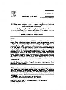
Figure 1: Squared loss function 𝑙1 (𝑟), absolute deviation loss function 𝑙2 (𝑟), and smooth approximation function 𝑙3 (𝑟) with ℎ = 0.3.
where 𝑙1 (𝑟) = 𝑟2 with 𝑟 = 𝑦 − 𝑓(𝑥), and is a squared loss function, as shown in Figure 1. In the reproducing kernel Hilbert space H, we rewrite the optimization problem (4) as min 𝑓
1 2 𝐶 𝑛 𝑓H + ∑𝑙1 (𝑦𝑖 − 𝑓 (𝑥𝑖 )) . 2 2 𝑖=1
(5)
For the sake of simplicity, we can drop the bias 𝑏 without loss of generalization performance of SVR [21]. According to [21], the optimal function for (5) can be expressed as a linear combination of the kernel functions centering the training samples: 𝑛
𝑓 (𝑥) = ∑𝛼𝑖 𝑘 (𝑥, 𝑥𝑖 ) .
(6)
𝑖=1
𝑛
min
3
(2)
where 𝑒 = (1, 1, . . . , 1)⊤ , y = (𝑦1 , 𝑦2 , . . . , 𝑦𝑛 )⊤ , 𝐼𝑛 denotes 𝑛 × 𝑛 identity matrix, 𝐾 = (𝐾𝑖𝑗 )𝑛×𝑛 is the kernel matrix with 𝐾𝑖𝑗 = 𝑘(𝑥𝑖 , 𝑥𝑗 ) = 𝜙(𝑥𝑖 )⊤ 𝜙(𝑥𝑗 ), and 𝑘(⋅, ⋅) is the kernel function. By solving (2), the regressor can be gained as 𝑓 (𝑥) = 𝑤⊤ 𝜙 (𝑥) + 𝑏 = ∑𝛼𝑖 𝑘 (𝑥𝑖 , 𝑥) + 𝑏.
3.5
0 −2
2. Least Squares Support Vector Regression
min
4
(4)
Substituting (6) into (5), we have min 𝛼
1 ⊤ 𝐶 𝑛 𝛼 𝐾𝛼 + ∑𝑙1 (𝑦𝑖 − 𝐾𝑖 𝛼) , 2 2 𝑖=1
(7)
where 𝛼 = (𝛼1 , 𝛼2 , . . . , 𝛼𝑛 )⊤ and 𝐾𝑖 is the 𝑖th row of kernel matrix 𝐾.
3. Least Absolute Deviation SVR As mentioned, LS-SVR is sensitive to outliers and noises with the squared loss function 𝑙1 (𝑟) = 𝑟2 . When there exist outliers which are far away from the rest of samples, large errors will dominate SSE and the decision hyperplane of LS-SVR will severely deviate from the original position deteriorating the performance of LS-SVR. In this section, we propose an absolute deviation loss function 𝑙2 (𝑟) = |𝑟| to reduce the influence of outliers. This
Mathematical Problems in Engineering
3
phenomenon is graphically depicted in Figure 1, which shows the squared loss function 𝑙1 (𝑟) = 𝑟2 and the absolute deviation one 𝑙2 (𝑟) = |𝑟|, respectively. From the figure, the exaggerative effect of 𝑙1 (𝑟) = 𝑟2 at points with large errors, as compared with 𝑙2 (𝑟) = |𝑟|, is evident. The robust LAD-SVR model can be constructed as min 𝛼
𝑛 1 ⊤ 𝛼 𝐾𝛼 + 𝐶∑𝑙2 (𝑦𝑖 − 𝐾𝑖 𝛼) . 2 𝑖=1
(8)
However, 𝑙2 (𝑟) is not differentiable, and the associated optimization problem is difficult to be solved. Inspired by the Huber loss function [23], we propose the following loss function: if |𝑟| > ℎ, {|𝑟| , 𝑙3 (𝑟) = { 𝑟2 ℎ + , otherwise, { 2ℎ 2
(9)
(10)
Noticing that the objective function L(𝛼) of (10) is continuous and differentiable, (10) can be easily solved by Newton algorithm. At the 𝑡th iteration, we divide the training samples into two groups according to |𝑟𝑖𝑡 | ≤ ℎ and |𝑟𝑖𝑡 | > ℎ. Let 𝑆1 = {𝑖 | |𝑟𝑖𝑡 | ≤ ℎ} denote the index set of samples lying in the quadratic part of 𝑙3 (𝑟) and 𝑆2 = {𝑖 | |𝑟𝑖𝑡 | > ℎ} the index set of samples lying in the linear part of 𝑙3 (𝑟). |𝑆1 | and |𝑆2 | represent the number of samples in 𝑆1 and 𝑆2 ; that is, |𝑆1 | + |𝑆2 | = 𝑛. For the sake of clarity, we suppose that the two groups are arranged in the order of 𝑆1 and 𝑆2 . Furthermore, we define 𝑛 × 𝑛 diagonal matrices 𝐼1 and 𝐼2 , where 𝐼1 has the first |𝑆1 | entries being 1 and the others 0, and 𝐼2 has the entries from |𝑆1 | + 1 to |𝑆1 | + |𝑆2 | being 1 and the others 0. Then, we develop a Newton algorithm for (10). The gradient is 𝐶 𝐶 𝐼1 𝐾) 𝛼𝑡 − 𝐾 [ 𝐼1 y + 𝐶𝐼2 s] , ℎ ℎ
(11)
where y = (𝑦1 , . . . , 𝑦𝑛 )⊤ and s = (𝑠1 , . . . , 𝑠𝑛 )⊤ with 𝑠𝑖 = sgn(𝑟𝑖 ). The Hessian matrix at the 𝑡th iteration is 𝐻𝑡 = 𝐾 (𝐼𝑛 +
𝐶 𝐼 𝐾) . ℎ 1
(12)
The Newton step at the (𝑡 + 1)th iteration is −1
𝛼𝑡+1 = 𝛼𝑡 − (𝐻𝑡 ) ∇L (𝛼𝑡 ) −1 𝐶 𝐶 = (𝐼𝑛 + 𝐼1 𝐾) ( 𝐼1 y + 𝐶𝐼2 s) . ℎ ℎ
𝐶 −1 𝐶 𝐴 − 𝐴𝐾𝑆1 ,𝑆2 ). 𝐼1 𝐾) = ( ℎ ℎ 𝑂 𝐼|𝑆2 |
(14)
The computational complexity of 𝐴−1 is 𝑂((|𝑆1 |)3 ). Substituting (14) into (13), we obtain 𝛼
𝑡+1
𝐴 𝛼𝑡+1 𝑆1 [y|𝑆1 | − 𝐶𝐾𝑆1 ,𝑆2 s|𝑆2 | ] = 𝐶(ℎ ) = ( 𝑡+1 ) . 𝛼𝑆2 s|𝑆2 |
(15)
Having updated 𝛼𝑡+1 , we get the corresponding regressor 𝑓𝑡+1 (𝑥) = ∑𝛼𝑖𝑡+1 𝑘 (𝑥𝑖 , 𝑥) .
(16)
𝑖=1
The flowchart of implementing LAD-SVR is depicted as follows. Algorithm 1. LAD-SVR (Newton algorithm for LAD-SVR with absolute deviation loss function). Input: training set 𝑇 = {𝑥𝑖 , 𝑦𝑖 }𝑛𝑖=1 , kernel matrix 𝐾, and a small real number 𝜌 > 0. (1) Let 𝛼0 ∈ 𝑅𝑛 and calculate 𝑟𝑖0 = 𝑦𝑖 − 𝐾𝑖 𝛼0 , 𝑖 = 1, . . . , 𝑛. Divide training set into two groups according to |𝑟𝑖0 |. Set 𝑡 = 0.
4. Newton Algorithm for LAD-SVR
∇L (𝛼𝑡 ) = 𝐾 (𝐼𝑛 +
(𝐼𝑛 +
𝑛
where ℎ > 0 is the Huber parameter, and its shape is shown in Figure 1. It is verified that 𝑙3 (𝑟) is differentiable. For ℎ → 0, 𝑙3 (𝑟) approaches 𝑙2 (𝑟). Replacing 𝑙2 (𝑟) with 𝑙3 (𝑟) in (8), we obtain 𝑛 1 ⊤ L = 𝐾𝛼 + 𝐶 𝑙3 (𝑦𝑖 − 𝐾𝑖 𝛼) . 𝛼 min ∑ (𝛼) 𝛼 2 𝑖=1
Denote 𝐴 = (𝐼|𝑆1 | +(𝐶/ℎ)𝐾𝑆1 ,𝑆1 )−1 . The inverse of 𝐼𝑛 +(𝐶/ℎ)𝐼1 𝐾 can be calculated as follows:
(13)
(2) Rearrange the groups in the order of 𝑆1 and 𝑆2 ; adjust 𝐾 and y correspondingly. Solve ∇L(𝛼𝑡 ) by (11). If ‖∇L(𝛼𝑡 )‖ ≤ 𝜌, stop; or else, go to the next step. (3) Calculate 𝛼𝑡+1 by (15) and 𝑓𝑡+1 (𝑥) by (16). (4) Divide training set into two groups according to |𝑟𝑖𝑡+1 | = |𝑦𝑖 − 𝐾𝑖 𝛼𝑡+1 |. Let 𝑡 = 𝑡 + 1, and go to step (2).
5. Experiments In order to test the effectiveness of the proposed LAD-SVR, we conduct experiments on several datasets, including six artificial datasets and nine benchmark datasets, and compare it with LS-SVR. Gaussian kernel is selected as the kernel function in the experiments. All the experiments are implemented on Intel Pentium IV 3.00 GHz PC with 2 GB of RAM using Matlab 7.0 under Microsoft Windows XP. The linear system of equations in LS-SVR is realized by Matlab operation “\”. Parameters selection is a crucial issue for modeling with the kernel methods, because improper parameters, such as the regularization parameter 𝐶 and kernel parameter 𝜎, will severely affect the generalization performance of SVR. Grid search [2] is a simple and direct method, which conducts an exhaustive search on the parameters space with the validation minimized. In this paper, we employ grid search for searching their optimal parameters such that they can achieve best performance on the test samples. To evaluate the performances of the algorithms, we adopt the following four popular regression estimation criterions:
4
Mathematical Problems in Engineering Table 1: Experiment results on 𝑦 = sin(3𝑥)/(3𝑥).
Noise
Algorithm LS-SVR LAD-SVR LS-SVR LAD-SVR LS-SVR LAD-SVR LS-SVR LAD-SVR LS-SVR LAD-SVR LS-SVR LAD-SVR
Type I Type II Type III Type IV Type V Type VI
RMSE 0.0863 0.0455 0.0979 0.0727 0.0828 0.0278 0.0899 0.0544 0.2120 0.1861 0.1796 0.1738
root mean square error (RMSE) [24], mean absolute error (MAE), ratio between the sum squared error SSE and the sum squared deviation testing samples SST (SSE/SST) [25], and ratio between interpretable sum deviation SSR and SST (SSR/SST) [25]. These criterions are defined as follows.
MAE 0.0676 0.0364 0.0795 0.0607 0.0665 0.0223 0.0707 0.0439 0.1749 0.1554 0.1498 0.1391
Type I: 𝑦𝑖 =
SSE/SST 0.0720 0.0209 0.0944 0.0527 0.0664 0.0078 0.0772 0.0291 0.4268 0.3372 0.3112 0.2928
sin (3𝑥𝑖 ) + 𝛾𝑖 , 3𝑥𝑖
(1) RMSE =
sin (3𝑥𝑖 ) + 𝛾𝑖 , 3𝑥𝑖
2
− 𝑦̂𝑖 ) .
sin (3𝑥𝑖 ) + 𝛾𝑖 , 3𝑥𝑖
Type III: 𝑦𝑖 =
2 ̂𝑖 − 𝑦𝑖 )2 / ∑𝑚 (3) SSE/SST = ∑𝑚 𝑖=1 (𝑦 𝑖=1 (𝑦𝑖 − 𝑦) .
(4) SSR/SST =
2
− 𝑦)
/ ∑𝑚 𝑖=1 (𝑦𝑖
𝑥𝑖 ∈ [−4, 4] ,
𝛾𝑖 ∼ 𝑁 (0, 0.32 ) .
̂𝑖 |. (2) MAE = (1/𝑚) ∑𝑚 𝑖=1 |𝑦𝑖 − 𝑦
̂𝑖 ∑𝑚 𝑖=1 (𝑦
𝑥𝑖 ∈ [−4, 4] ,
𝛾𝑖 ∼ 𝑁 (0, 0.152 ) . Type II: 𝑦𝑖 =
√(1/𝑚) ∑𝑚 𝑖=1 (𝑦𝑖
SSR/SST 1.0761 1.0082 0.9374 1.0224 1.1137 1.0044 0.9488 1.0003 0.7142 0.7291 0.9709 0.8993
2
− 𝑦) ,
where 𝑚 is the number of testing samples, 𝑦𝑖 denotes the target, 𝑦̂𝑖 is the corresponding prediction, and 𝑦 = (1/𝑚) ∑𝑚 𝑖=1 𝑦𝑖 . RMSE is commonly used as the deviation measurement between the real and predicted values. It represents the fitting precision. The smaller RMSE is, the better fitting performance is. However, when noises are also used as testing samples, too small value of RMSE probably means overfitting of the regressor. MAE is also a popular deviation measurement between the real and predicted values. In most cases, small SSE/SST indicates good agreement between estimations and real values. Obtaining smaller SSE/SST usually accompanies an increase in SSR/SST. However, the extremely small value of SSE/SST is in fact not good, for it probably means overfitting of the regressor. Therefore, a good estimator should strike balance between SSE/SST and SSR/SST. 5.1. Experiments on Artificial Datasets. In artificial experiments, we generate the artificial datasets {(𝑥𝑖 , 𝑦𝑖 )}𝑛𝑖=1 by the following Sinc function which is widely used in regression estimation [17, 24]. Consider
𝑥𝑖 ∈ [−4, 4] ,
𝛾𝑖 ∼ 𝑈 [−0.15, 0.15] . sin (3𝑥𝑖 ) + 𝛾𝑖 , 3𝑥𝑖
Type IV: 𝑦𝑖 =
(17)
𝑥𝑖 ∈ [−4, 4] ,
𝛾𝑖 ∼ 𝑈 [−0.3, 0.3] . Type V: 𝑦𝑖 =
sin (3𝑥𝑖 ) + 𝛾𝑖 , 3𝑥𝑖
𝑥𝑖 ∈ [−4, 4] , 𝛾𝑖 ∼ 𝑇 (4) .
Type VI: 𝑦𝑖 =
sin (3𝑥𝑖 ) + 𝛾𝑖 , 3𝑥𝑖
𝑥𝑖 ∈ [−4, 4] , 𝛾𝑖 ∼ 𝑇 (8) ,
where 𝑁(0, 𝑑2 ) represents the Gaussian random variable with zero means and variance 𝑑2 , 𝑈[𝑎, 𝑏] denotes the uniformly random variable in [𝑎, 𝑏], and 𝑇(𝑐) depicts the student random variable with freedom degree 𝑐. In order to avoid biased comparisons, for each kind of noises, we randomly generate ten independent groups of noisy samples which, respectively, consist of 350 training samples and 500 test samples. For each training dataset, we randomly choose 1/5 samples and add large noise on their
Mathematical Problems in Engineering
5
2 1.5 1 0.5 0 −0.5 −1 −1.5 −2 −2.5 −4
−3
−2
−1
0
1
2
3
4
2.5 2 1.5 1 0.5 0 −0.5 −1 −1.5 −2 −2.5 −4
−3
−2
−1
(a)
2
1.5
1.5
1
1
0.5
0.5
0
0
−0.5
−0.5
−1
−1
−1.5
−1.5
−2
−2
−2.5 −4
−2.5 −4
−2
−1
0
1
2
3
4
−3
−2
−1
(c)
2
3
4
0
1
2
3
4
(d)
6
6
4
4
2
2
0
0
−2
−2
−4
−4
−6 −8 −4
1
(b)
2
−3
0
−3
−2
−1
0
1
2
3
4
LS-SVR LAD-SVR
Samples Sinc(x) (e)
−6 −4
−3
−2
−1
0
1
2
3
4
LS-SVR LAD-SVR
Samples Sinc(x) (f)
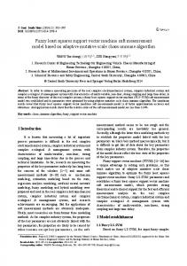
Figure 2: Experiment results on 𝑦 = sin(3𝑥)/(3𝑥) with noise of Type I(a), II(b), . . ., VI(f).
targets to simulate outliers. The testing samples are uniformly from the objective Sinc function without any noise. Table 1 shows the average accuracies of LS-SVR and LAD-SVR with ten independent runs. From Table 1, we can see that LADSVR has advantages over LS-SVR for all types of noises in terms of RMSE, MAE, and SSE/SST. Hence, LAD-SVR is robust to noises and outliers. Moreover, LAD-SVR derives larger SSR/SST value for three types of noises (types II, IV, and V). From Figure 2, we can see that the LAD-SVR follows the actual data more closely than LS-SVR for most of the test samples. The main reason is that LAD-SVR employs an absolute deviation loss function which reduces the penalty of outliers in the training process. The histograms of LSSVR and LAD-SVR for distribution of the error variables
𝜉𝑖 for these different types of noises are shown in Figure 3. We notice that the histograms of LAD-SVR for all types of noises are closer to Gaussian distribution, compared with LS-SVR. Therefore, our proposed LAD-SVR derives better approximation than LS-SVR. 5.2. Experiments on Benchmark Datasets. In this section, we test nine benchmark datasets to further illustrate the effectiveness of the LAD-SVR, including Pyrimidines (Pyrim), Triazines, AutoMPG, Boston Housing (BH) and Servo from UCI datasets [26], Bodyfat, Pollution, Concrete Compressive Strength (Concrete) from StatLib database (Available from http://lib.stat.cmu.edu/datasets/), and Machine CPU
6
Mathematical Problems in Engineering 140
100
120 100
60 40
80
Freq.
Freq.
Freq.
80
60 40
20 0 −2
90
20 −1
0
1
0 −2
2
−1
𝜉i
0
80
80
70
70
60
60
50
50
40
30
20
20
10
10 −1
0
1
120
0 −2
60
0
1
0
2
−2
−1
𝜉i
60
50 40
0
1
30
20
20
10
10
0
2
−2
−1
0
70
80
60 Freq.
Freq.
Freq.
50 40 30 20
10
10 −5
0
5
10
0 −10
−5
0
5
10
𝜉i
𝜉i
−2 −1
0
1
2
𝜉i
𝜉i
70
20
0 −10
0
2
(e)
70
70
60
60
50
50
40
40
Freq.
90
30
1
(d)
80
40
50 40
(c)
50
2
80
𝜉i
60
1
70
30
20 −1
90
Freq.
80
40
20
100
80
60 Freq.
Freq.
Freq.
40
90
70
100
60
0
(b)
140
80
−1
𝜉i
(a)
100
0 −2
2
𝜉i
𝜉i
120
40
30
0 −2
2
1
90
Freq.
120
30
30
20
20
10
10
0
−5
0
5
𝜉i
0
−5
0
5
𝜉i (f)
Figure 3: Histograms of distribution of the error variables 𝜉𝑖 for noise of Type I ((a) LS-SVR (Left), LAD-SVR (Right)), II(b), . . ., VI(f).
(MCPU) from the web page (http://www.dcc.fc.up.pt/∼ ltorgo/Regression/DataSets.html), which are widely used in evaluating various regression algorithms. The detailed descriptions of datasets are presented in Table 2, where #train
and #test denote the number of training and testing samples, respectively. In experiments, each dataset is randomly split into training and testing samples. For each training dataset, we randomly choose 1/5 samples and add large noise on their
Mathematical Problems in Engineering
7
Table 2: Experiment results on Benchmark datasets. Number 1 2 3 4 5 6 7 8 9
Dataset Bodyfat (252 × 14) Pyrim (74 × 27) Pollution (60 × 16) Triazines (186 × 60) MCPU (209 × 6) AutoMPG (392 × 7) BH (506 × 13) Servo (167 × 4) Concrete (1030 × 8)
Algorithm LS-SVR LAD-SVR LS-SVR LAD-SVR LS-SVR LAD-SVR LS-SVR LAD-SVR LS-SVR LAD-SVR LS-SVR LAD-SVR LS-SVR LAD-SVR LS-SVR LAD-SVR LS-SVR LAD-SVR
RMSE 0.0075 0.0026 0.1056 0.1047 39.8592 36.1070 0.1481 0.1415 53.6345 50.2263 2.8980 2.6630 4.3860 3.6304 0.7054 0.6830 7.0293 6.8708
MAE 0.0056 0.0012 0.0649 0.0641 31.0642 28.2570 0.1126 0.1066 27.5341 26.5241 2.1601 1.9208 3.2163 2.5349 0.4194 0.3767 5.1977 5.0748
targets to simulate outliers. Similar to the experiments on artificial datasets, the testing datasets are not added any noise on their targets. All the regression methods are repeated ten times with different partition of training and testing dataset. Table 2 displays the testing results of LS-SVR and the proposed LAD-SVR. We observe that the three criterions (RMSE, MAE, and SSE/SST) of LAD-SVR are obviously better than LS-SVR on all datasets, which shows that the robust algorithm achieves better generalization performance and has good stability as well. Moreover, our LAD-SVR algorithm outperforms LS-SVR. For instance, LAD-SVR obtains the smaller RMSE, MAE, and SSE/SST on the Bodyfat dataset; meanwhile, it keeps larger SSR/SST than LS-SVR. The proposed algorithm derives the similar results on the MCPU, AutoMPG, and BH datasets. To obtain the final regressor of LAD-SVR, the resultant model is implemented in the primal space by classical Newton algorithm iteratively. The number of iterations (Iter) and the running time (Time) including the training and testing time are listed in Table 2. Iter shows the average number of iterations of ten independent runs. Compared with LS-SVR, LAD-SVR requires more running time. The main reason is that the running time of LAD-SVR is affected by the selection approach of the starting point 𝛼0 , the value of |𝑆1 |, and the number of iterations. In the experiments, the starting point 𝛼0 is derived by LS-SVR on a small number of training samples. It can be observed that the average number of iterations does not exceed 10, which implies that LAD-SVR is suitable enough for medium and large scale problems. We notice that LAD-SVR does not burden the running time severely. A worse case is that the maximum ratio of their speeds is no more than 3 times on Pyrim dataset. These experimental results conclude that the proposed LAD-SVR is effective in dealing with robust regression problems.
SSE/SST 0.1868 0.0277 0.5925 0.5832 0.5358 0.4379 0.9295 0.8420 0.1567 0.1364 0.1308 0.1102 0.2402 0.1648 0.2126 0.2010 0.1740 0.1662
SSR/SST 0.7799 0.9686 0.5729 0.5342 0.8910 0.7312 0.3356 0.3026 0.9485 0.9666 0.8421 0.8502 0.8563 0.8593 0.8353 0.8147 0.9005 0.8936
Time (s) 0.0854 0.0988 0.0137 0.0385 0.0083 0.0202 0.0759 0.0958 0.0509 0.0883 0.2916 0.3815 0.2993 0.4971 0.0342 0.0561 1.1719 2.0737
Iter / 4.4 / 9.8 / 5 / 6 / 5.4 / 6.4 / 8.8 / 4.9 / 8.7
#train 200 200 50 50 40 40 150 150 150 150 300 300 300 300 100 100 500 500
#test 52 52 24 24 20 20 36 36 59 59 92 92 206 206 67 67 530 530
6. Conclusion In this paper, we propose LAD-SVR, a novel robust least squares support vector regression algorithm on dataset with outliers. Compared with the classical LS-SVR which is based on squared loss function, LAD-SVR employs an absolute deviation loss function to reduce the influence of outliers. To solve the resultant model, we smooth the proposed loss function by a Huber loss function and develop a Newton algorithm. Experimental results on both artificial datasets and benchmark datasets confirm that LAD-SVR owns better robustness compared with LS-SVR. However, LAD-SVR still loses sparseness as LS-SVR. In the future, we plan to develop more efficient LAD-SVR to improve the sparseness and robustness.
Conflict of Interests The authors declare that there is no conflict of interests regarding the publication of this paper.
Acknowledgments The work is supported by the National Natural Science Foundation of China under Grant no. 11171346 and Chinese Universities Scientific Fund no. 2013YJ010.
References [1] V. Vapnik, The Nature of Statistical Learning Theory, Springer, New York, NY, USA, 1995. [2] N. Cristianini and J. S. Taylor, An Introduction to Support Vector Machines and Other Kernel-Based Learning Methods, Cambridge University Press, Cambridge, UK, 2000.
8 [3] S. S. Keerthi, S. K. Shevade, C. Bhattacharyya, and K. R. K. Murthy, “Improvements to Platt’s SMO algorithm for SVM classifier design,” Neural Computation, vol. 13, no. 3, pp. 637– 649, 2001. [4] J. Platt, “Fast training of support vector machines using sequential minimal optimization,” in Advances in Kernel Methods: Support Vector Learning, B. Sch¨olkopf, C. J. C. Burges, and A. J. Smola, Eds., pp. 185–208, MIT Press, Cambridge, UK, 1999. [5] E. Osuna, R. Freund, and F. Girosi, “An improved training algorithm for support vector machines,” in Proceedings of the 7th IEEE Workshop on Neural Networks for Signal Processing (NNSP ’97), J. Principe, L. Gile, N. Morgan, and E. Wilson, Eds., pp. 276–285, September 1997. [6] T. Joachims, “Making large-scale SVM learning practical,” in Advances in Kernel Methods-Support Vector Learning, B. Sch¨olkopf, C. J. C. Burges, and A. J. Smola, Eds., pp. 169–184, MIT Press, Cambridge, Mass, USA, 1999. [7] C. Chang and C. Lin, “LIBSVM: a library for support vector machines,” 2001, http://www.csie.ntu.edu.tw/∼cjlin/. [8] J. A. K. Suykens and J. Vandewalle, “Least squares support vector machine classifiers,” Neural Processing Letters, vol. 9, no. 3, pp. 293–300, 1999. [9] J. A. K. Suykens, J. De Brabanter, L. Lukas, and J. Vandewalle, “Weighted least squares support vector machines: robustness and sparce approximation,” Neurocomputing, vol. 48, pp. 85– 105, 2002. [10] W. Wen, Z. Hao, and X. Yang, “A heuristic weight-setting strategy and iteratively updating algorithm for weighted leastsquares support vector regression,” Neurocomputing, vol. 71, no. 16-18, pp. 3096–3103, 2008. [11] K. De Brabanter, K. Pelckmans, J. De Brabanter et al., “Robustness of kernel based regression: acomparison of iterative weighting schemes,” in Proceedings of the 19th International Conference on Artificial Neural Networks (ICANN ’09), 2009. [12] J. Liu, J. Li, W. Xu, and Y. Shi, “A weighted 𝐿𝑞 adaptive least squares support vector machine classifiers-Robust and sparse approximation,” Expert Systems with Applications, vol. 38, no. 3, pp. 2253–2259, 2011. [13] X. Chen, J. Yang, J. Liang, and Q. Ye, “Recursive robust least squares support vector regression based on maximum correntropy criterion,” Neurocomputing, vol. 97, pp. 63–73, 2012. [14] L. Xu, K. Crammer, and D. Schuurmans, “Robust support vector machine training via convex outlier ablation,” in Proceedings of the 21st National Conference on Artificial Intelligence (AAAI ’06), pp. 536–542, July 2006. [15] P. J. Rousseeuw and K. van Driessen, “Computing LTS regression for large data sets,” Data Mining and Knowledge Discovery, vol. 12, no. 1, pp. 29–45, 2006. [16] W. Wen, Z. Hao, and X. Yang, “Robust least squares support vector machine based on recursive outlier elimination,” Soft Computing, vol. 14, no. 11, pp. 1241–1251, 2010. [17] C. Chuang and Z. Lee, “Hybrid robust support vector machines for regression with outliers,” Applied Soft Computing Journal, vol. 11, no. 1, pp. 64–72, 2011. [18] G. Bassett Jr. and R. Koenker, “Asymptotic theory of least absolute error regression,” Journal of the American Statistical Association, vol. 73, no. 363, pp. 618–622, 1978. [19] P. Bloomfield and W. L. Steiger, Least Absolute Deviation: Theory, Applications and Algorithms, Birkhauser, Boston, Mass, USA, 1983.
Mathematical Problems in Engineering [20] H. Wang, G. Li, and G. Jiang, “Robust regression shrinkage and consistent variable selection through the LAD-Lasso,” Journal of Business & Economic Statistics, vol. 25, no. 3, pp. 347–355, 2007. [21] O. Chapelle, “Training a support vector machine in the primal,” Neural Computation, vol. 19, no. 5, pp. 1155–1178, 2007. [22] L. Bo, L. Wang, and L. Jiao, “Recursive finite Newton algorithm for support vector regression in the primal,” Neural Computation, vol. 19, no. 4, pp. 1082–1096, 2007. [23] P. J. Huber, Robust Statistics, Springer, Berlin, Germany, 2011. [24] P. Zhong, Y. Xu, and Y. Zhao, “Training twin support vector regression via linear programming,” Neural Computing and Applications, vol. 21, no. 2, pp. 399–407, 2012. [25] X. Peng, “TSVR: an efficient Twin Support Vector Machine for regression,” Neural Networks, vol. 23, no. 3, pp. 365–372, 2010. [26] C. Blake and C. J. Merz, “UCI repository for machine learning databases,” 1998, http://www.ics.uci.edu/∼mlearn/MLRepository.html.
Advances in
Operations Research Hindawi Publishing Corporation http://www.hindawi.com
Volume 2014
Advances in
Decision Sciences Hindawi Publishing Corporation http://www.hindawi.com
Volume 2014
Journal of
Applied Mathematics
Algebra
Hindawi Publishing Corporation http://www.hindawi.com
Hindawi Publishing Corporation http://www.hindawi.com
Volume 2014
Journal of
Probability and Statistics Volume 2014
The Scientific World Journal Hindawi Publishing Corporation http://www.hindawi.com
Hindawi Publishing Corporation http://www.hindawi.com
Volume 2014
International Journal of
Differential Equations Hindawi Publishing Corporation http://www.hindawi.com
Volume 2014
Volume 2014
Submit your manuscripts at http://www.hindawi.com International Journal of
Advances in
Combinatorics Hindawi Publishing Corporation http://www.hindawi.com
Mathematical Physics Hindawi Publishing Corporation http://www.hindawi.com
Volume 2014
Journal of
Complex Analysis Hindawi Publishing Corporation http://www.hindawi.com
Volume 2014
International Journal of Mathematics and Mathematical Sciences
Mathematical Problems in Engineering
Journal of
Mathematics Hindawi Publishing Corporation http://www.hindawi.com
Volume 2014
Hindawi Publishing Corporation http://www.hindawi.com
Volume 2014
Volume 2014
Hindawi Publishing Corporation http://www.hindawi.com
Volume 2014
Discrete Mathematics
Journal of
Volume 2014
Hindawi Publishing Corporation http://www.hindawi.com
Discrete Dynamics in Nature and Society
Journal of
Function Spaces Hindawi Publishing Corporation http://www.hindawi.com
Abstract and Applied Analysis
Volume 2014
Hindawi Publishing Corporation http://www.hindawi.com
Volume 2014
Hindawi Publishing Corporation http://www.hindawi.com
Volume 2014
International Journal of
Journal of
Stochastic Analysis
Optimization
Hindawi Publishing Corporation http://www.hindawi.com
Hindawi Publishing Corporation http://www.hindawi.com
Volume 2014
Volume 2014