Linear Parametric Noise Models for Least Squares Support Vector ...

Linear Parametric Noise Models for Least Squares Support Vector Machines Tillmann Falck, Johan A.K. Suykens and Bart De Moor Abstract—In the identification of nonlinear dynamical models it may happen that not only the system dynamics have to be modeled but also the noise has a dynamic character. We show how to adapt Least Squares Support Vector Machines (LSSVMs) to take advantage of a known or unknown noise model. We furthermore investigate a convex approximation based on overparametrization to estimate a linear auto regressive noise model jointly with a model for the nonlinear system. Considering a noise model can improve generalization performance. We discuss several properties of the proposed scheme on synthetic data sets and finally demonstrate its applicability on real world data.

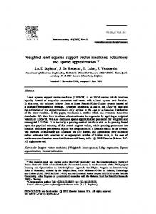
I. I NTRODUCTION The objective in system identification [1] of nonlinear systems [2], [3] is to estimate a model for a dynamical system from observational data. In linear as well as in nonlinear systems, model structures are of particular interest as they are crucial for the flexibility of the model to explain data. In nonlinear systems NARX and NFIR structures are most used as the corresponding estimation problems are linear in the parameters. Then the estimation is convex, if a conex objective is used. Generalizations of more advanced model structures like ARMAX or Box-Jenkins (BJ) to nonlinear systems exist but even in a linear setting the identification is a non convex problem. In this paper we consider NARX models extended by a linear ARMA model for the noise. This structure is depicted in Figure 1. We will denote this hybrid structure as ARMA-NARX. Note that in a NARMAX model the estimated noise is used as an additional input to the nonlinear system and thus can have nonlinear dynamics. The ARMA-NARX model is simply tailored towards colored noise instead of assuming a white spectrum as in NARX models. We consider two cases: • In the first case we assume that the noise model is known. This information can be easily integrated into the estimation problem and can improve the performance of the resulting model. This approach has already been explored in [4]. In [4] the noise model is tuned as hyperparameters of the nonlinear model, if it is not known a priori. In this part, we restrict ourselves to generalize the results from AR to ARMA models. • The second case jointly estimates an AR noise model and the NARX part. This is a nonconvex, nonlinear problem. The main contribution of this paper is to Tillmann Falck, Johan Suykens and Bart De Moor are with the SCD group of the Department of Electrical Engineering (ESAT), Katholieke Universiteit Leuven, Kasteelpark Arenberg 10, B-3001 Leuven (Heverlee), Belgium. Email: {tillmann.falck,johan.suykens,bart.demoor}@esat.kuleuven.be

rt H(z) et

ut

yˆt

NARX

+ +

yt

yt−1 z −1 Fig. 1: Block diagram of a nonlinear model (Du = 0, Dy = 1) consisting of a NARX part and a linear noise model. Here denoted as ARMA-NARX.

propose a convex relaxation to this problem. This complements [4] with an effective way to obtain estimates for unknown noise models. The relaxation is based on the overparametrization technique [11], [12]. It was introduced for a special class of structured nonlinear systems called Hammerstein systems. The idea is to relax non-convex bilinear products by replacing them with new independent variables. This leads to a convex formulation and in the context of identification of Hammerstein systems using LS-SVMs has been successfully applied in [13], [14]. To model the nonlinear system we employ Least Squares Support Vector Machines (LS-SVMs) which is based on the methodology of Support Vector Machines (SVMs) [5], [6]. Both belong to the class of kernel based models, which also includes e.g. Splines [7] and Gaussian Processes [8]. In LS-SVM the inequality constraints of SVMs are replaced by equality constraints and the L1 -loss on the residuals by the sum of squares. For regression problems this has the advantage that it can be solved by a linear system instead of a QP. Disadvantages of this scheme are the non-sparse solution and no inherent robustness. Especially for large scale data sets sparsity can be obtained by approximating the feature map on a subsample and then solving the primal problem. This is called Fixed-Size LS-SVM [9]. If needed robustness can be achieved by reweighting the residuals [10]. This paper is structured as follows. In Section II we show how to integrate a known ARMA noise model with a LSSVM based nonlinear model. The joint convex estimation of an AR(P) noise model with the nonlinear model based on overparametrization is covered in Section III. Experimental results on synthetic as well as real data illustrating the pro-

posed scheme are given in IV. Finally the paper is concluded in Section V. II. I NCORPORATING LINEAR NOISE MODELS IN LS-SVM S A. LS-SVM regression D Consider observational data {xt , yt }N t=1 with xt ∈ R and yt ∈ R where xt = [yt−1 , . . . , yt−Dy , ut , . . . , ut−Du ]T and D = Du + Dy . ut , yt are respectively input and output measurements of a nonlinear system S and t denotes the time index. Then a nonlinear dynamical model for S can be estimated using least squares support vector machine (LSSVM) regression [9] N 1 X 2 1 T w w+ γ e w,b,et 2 2 t=1 t subject to yt = wT ϕ(xt ) + b + et ,

min

(P-0) t = 1, . . . , N

with the feature map ϕ : RD → Rnh and the parameter vector w ∈ Rnh . Here we use equation numbers of the form (P-x) and (D-x) to denote a primal optimization problem and its dual. Note that not all dual formulations are given explicitly. The predictive model for (P-0) is given by yˆ = wT ϕ(x) + b. The dual model is yˆ =

N X

αt K(xt , x) + b

(1)

t=1

respectively. It can be derived using Lagrangian duality and by applying the kernel trick to replace inner products of the feature map with a the kernel function K(xi , xj ) = ϕ(xi )T ϕ(xj ). Least squares estimation is optimal for Gaussian white noise et . The problem as stated above is convex in its parameters w, et and b and can be solved as a linear system. To obtain a model with good generalization performance model selection is crucial. The model is defined the regularization parameter γ and possibly one or more parameters of the feature map/kernel function. The selection of model parameters is usually done by a validation criterion e.g. cross-validation [15]. In this paper we will discuss noise models, i.e. situations where et is not white. We show how to incorporate an a priori known linear noise model for et to improve the estimation and a propose scheme to estimate a noise model. B. Parametric noise models Define the backshift operator in time z −1 as z −1 et = et−1 . Consider a minimum phase noise model for et in transfer function form A(z)et = B(z)rt where rt is a white noise sequence, A(z) = 1 + a1 z −1 + · · · + aP z −P and B(z) = b0 + b1 z −1 + · · · + bQ z −Q . For the sake of simplicity we will assume for the rest of the paper that P = Q. Assuming that A(z) and B(z) are known apriori, the optimal LS-SVM

based model is obtained by solving

min

w,b,et ,rt

N 1 X 2 1 T w w+ γ rt 2 2 t=P +1

subject to yt = wT ϕ(xt ) + b + et , A(z)et = B(z)rt ,

t = P + 1, . . . , N t = P + 1, . . . , N. (P-1) If A(z) and B(z) are not known a priori, they can be seen as additional hyper-parameters to the problem, which have to be selected for example by cross-validation. In case A(z) and B(z) correspond to the true noise model the residual rt is white and the formulation becomes optimal. The values of rt and et for t = 1, . . . , P are the initial conditions for the noise model and are assumed to be zero. The constraint A(z)et = B(z)rt for t = P + 1, . . . , N with zero initial conditions can be written in matrix notation as Ae = Br with 

 1 a1 1    a2 a1 1  A=  ∈ RN ×N ,  ..  . ..   . aP ··· 1   b0 b1 b0    b2 b1 b0  B=  ∈ RN ×N ,  ..  . ..   . bP ··· b0 e = [e1 , . . . , eN ]T and r = [r1 , . . . , rN ]T . Proposition 1: Solving (P-0) with weighted residuals [10] eT De and D = AT B −T B −1 A instead of eT e is equivalent to solving (P-1) with zero initial conditions. The solution to the weighted problem is given by the linear system      y Ω + γ −1 D −1 1 α = (D-1) 0 1T 0 b in terms of the dual variables α and with Ωij = K(xi , xj ). Proof: For b0 6= 0 the matrix B is invertible, therefore the noise model can be rewritten as r = B −1 Ae. Substitution of this relation into the objective function of (P-1) yields the weighting matrix D. Note that A is also invertible and thus D as well. This is needed for the solution in the dual domain. Deriving the dual system relies on Lagrangian duality and the kernel trick K(xi , xj ) = ϕ(xi )T ϕ(xj ). For details consult [10]. Remark 1: The nonlinear model yt = wT ϕ(xt ) + b + et can also be solved for et . Then substitution into A(z)et =

B(z)rt yields a new combined modeling equation

yt = wT ϕ(xt ) +

P X

problem min

ak wT ϕ(xt−k ) + ¯b

w,b,ak ,et ,rt

k=1

−

P X

ak yt−k + B(z)rt

(2)

k=1

N 1 X 2 1 T w w+ γ rt 2 2 t=P +1

subject to yt = wT ϕ(xt ) + b + et , t = 1, . . . , N, P X et = ak et−k + rt , t = P + 1, . . . , N. k=1

PP with ¯b = b(1 + k=1 ak ). This relation can be written more compactly using matrix notation as Ay = AΦT w + bA1 + Br where Φ = [ϕ(x1 ), . . . , ϕ(xN )]. Then the dual system for the problem (P-1), with (2) replacing the model constraints, is  AΩAT + γ −1 BB T 1T A T

A1 0

    β Ay = . b 0

(D-10 )

Note that no explicit inverse is needed in this formulation. The kernel matrix is replaced by an equivalent kernel matrix AΩAT . In [4] also the model is expressed in terms of an equivalent kernel matrix Keq (xj , xi ) = PP k,l=0 ak al K(xi−k , j − l) with a0 = 1. The model can then be evaluated at a new point by

(P-2) The nonconvexity is due to the bilinear term ak et−k . Based on the idea of overparametrization [11], [12] we propose a convex approximation to (P-2). In a first step eliminate et as done in (2). In the new expression the nonconvexity is now contained in bilinear terms ak w. The idea of overparametrization is to replace these terms by new variables wk = ak w, k = 1, . . . , P . For ease of notation and clarity we will additionally define w0 = a0 w where a0 = 1. Then a convex relaxation to (P-2) can be written as min

wk ,¯ b,ak ,rt

N P 1 X 2 1X T rt wk wk + γ 2 2 t=P +1

k=0

subject to P X wTk ϕ(xt−k ) + ¯b + rt k=0

yˆt = f (yt−1 , . . . , yt−P , xt , . . . , xt−P ) =

N X n=P +1

αt Keq (xn , xt ) + ¯b −

P X

= yt + ak yt−k . (3)

k=1

For a model with good generalization performance model selection is needed. If the parameters ap and bq of the noise model are not known apriori, they have to be included in the model selection. In that case the regularization parameter γ, parameters of the kernel function and the noise model coefficients have to be tuned according to a validation scheme. This is computationally very demanding for all but very low order noise models. In the next section we propose a convex relaxation, that is able to estimate the noise model coefficients jointly with the parameters of the nonlinear model w and b.

P X

ak yt−k ,

t = P + 1, . . . , N.

k=1

(P-3) To fully recover the original problem in (P-2) a rank constraint rank([w0 , ..., wP ]) = 1 on the newly introduced variables would have to be included in the problem. This rank constraint captures the nonconvexity of (P-2) and the convex approximation is then achieved by simply dropping it from the problem. For LS-SVMs this technique has been successfully applied for the identification of Hammerstein systems in [13], [14]. B. Solution in dual domain

A. Primal model

In support vector machines the feature map ϕ is implicitly defined by a positive semidefinite kernel function K(·, ·). Depending on the choice of the kernel function the feature map can be infinite dimensional, as it is the case for the widely used RBF kernel KRBF (x, y) = exp(−kx−yk2 /σ 2 ). To obtain a finite dimensional solution in terms of the kernel function the Lagrange dual is computed and the kernel trick is applied to replace inner products of the feature map ϕ(x)T ϕ(y) by the kernel function K(x, y). The final solution is formalized in the following Lemma. Lemma 1: The solution of (P-3) in the dual is given by PP     1 Y 1 α y0 k=0 Ωk + γ I T      a 0 = (D-3) Y 0 0 ¯ T b 0 1 0 0

Therefore we consider the problem of jointly estimating the nonlinear model and a linear parametric noise model. This is formalized in the following nonconvex optimization

with (Ωk )ij = K(xi−k , xj−k ), P + 1 ≤ i, j ≤ N where (Ωk )ij is the ij-th element of Ωk . Furthermore α are the Lagrange multipliers corresponding to the equality

III. E STIMATION OF PARAMETRIC NOISE MODELS In the following we will only consider purely autoregressive models of order P (AR(P ) noise models) i.e. B(z) = 1. This simplifies the estimation problem as the nonconvex product of unknowns bq rt−q do not have to be considered. It also simplifies the prediction as the sequence rt does not have to estimated.

constraints, y k = [yP +1−k , . . . , yN −k ]T for k = 0, . . . , P and Y = [y 1 , . . . , y P ]. In the following we will use ˆ LS = [1, a ˆ T ]T to denote the estimate for ak resulting from a (D-3). Proof: The Lagrangian for (P-3) is P N 1X T 1 X 2 wk wk + γ rt L (wk , ¯b, ak , rt , α) = 2 2 t=P +1

k=0

−

N X

αt

t=P +1

P X

wTk ϕ(xt−k ) + ¯b + rt

k=0

−

P X

αT ΩP 0 α · · ·

! ak yt−k − yt

. (4)

k=1

Taking the Karush-Kuhn-Tucker (KKT) conditions [16] for optimality one obtains N X ∂L : wk = αt ϕ(xt−k ), ∂wk

k = 0, . . . , P,

(5a)

t=P +1

∂L : ∂¯b

N X

αt = 0,

(5b)

t=P +1

∂L : γrt = αt , t = P + 1, . . . , N, ∂rt N X ∂L : αt yt−k = 0, k = 1, . . . , P, ∂ak

(5c) (5d)

t=P +1

P

P

X X ∂L : yt = wTk ϕ(xt−k ) + ¯b + rt − ak yt−k , ∂αt k=0

k=1

t = P + 1, . . . , N. (5e) Substitution of (5a) and (5c) into ∂L /∂αt = 0 yields P N X X

αn K(xn−k , xt−k ) + ¯b + αt = yt +

k=0 n=P +1

P X

ak yt−k

k=1

after applying the kernel trick K(xn−k , xt−k ) = ϕ(xn−k )T ϕ(xt−k ). Expressing this, (5b) and (5d) in matrix notation yields (D-3). Remark 2: Evaluating the overparametrized model in terms of the dual variables α and primal variables ¯b and {ak }P k=1 is done using the one step ahead predictor yˆt = f (yt−1 , . . . , yt−P , xt , . . . , xt−P ) =

N X n=P +1

αn

P X

¯ K(xtrain n−k , xt−k ) + b −

k=0

P X

Gaussian RBF kernel this matrix has an infinite number of rows. Therefore consider the matrix W T W and its eigenvalue decomposition W T W = V S 2 V T to recover the rank-1 structure. Using the KKT conditions (5a) for wk the columns of W can be expressed in terms of the dual variables α. Then the finite dimensional matrix can be computed by applying the kernel trick on all elements of the matrix. This yields   T α Ω00 α · · · αT Ω0P α   .. .. .. (7) WTW =   . . .

ak yt−k . (6)

k=1

αT ΩP P α

with (Ωkl )ij = K(xi−k , xj−l ) for k, l = 0, . . . , P and i, j = P + 1, . . . , N . Now let s0 ≥ s1 ≥ · · · ≥ sP ≥ 0 be the orderd sequence of singular values of W such that S = diag(s0 , . . . , sP ) and denote the corresponding right singular vectors by v k . Both can be obtained from the eigenvalue decomposition of W T W . Then an estimate for a can be obtained as ˆ SVD = v 0 /(v 0 )0 . Using this estimate a complete model a can be estimated by solving (P-1). Remark 3: The projection onto the class of AR(P)-LSSVM is incomplete as two independent estimates for ak are obtained, one following directly from the solution of the dual system (D-3) and the other from the rank one approximation of W as outlined in this section. Therefore we compare the performance of an AR(P)-LS-SVM model based on both estimates in the experimental section. Algorithm 1 Overparametrized model (OVER) Training: PP 1. compute kernel matrix Ω = k=0 Ωk 2. solve (D-3) to obtain estimates for α, b and a Prediction: Estimates are generated according to (6)

Algorithm 2 AR(P) model with direct estimate for the noise model (DIRECT) Training: PP 1. compute kernel matrix Ω = k=0 Ωk 2. solve (D-3) to obtain estimates for α, b and a, denote ˆ LS the estimate for a by a ˆ LS 3. compute final model by solving (P-1) given a Prediction: Estimates are generated according to (3)

C. Projection onto true model class The model obtained from (D-3) is only an approximation for the AR(P)-LS-SVM model stated in (P-2). The overparametrized model needs to be projected to recover the AR(P) model structure. The approximation stems from dropping the rank-1 constraint on W = [w0 , . . . , wP ]. In presence of the rank-1 constraint the solution could be expressed as the outer product W = waT . For the popular

This results in three possible algorithms to obtain a predictive model. The first possibility is described in Algorithm 1 and uses the overparametrized model for projections. The second model uses the direct estimate for a to estimate an AR(P) model as explained in Alg. 2. Finally another AR(P) model can be obtained by using the estimate for a obtained from the projection. This is outlined in Alg. 3.

0.8 RMSE on validation set

Algorithm 3 AR(P) model with projection based estimate for the noise model (SVD) Training: PP 1. compute kernel matrix Ω = k=0 Ωk 2. solve (D-3) to obtain estimates for α, b and a 3. compute W T W according to (7) 4. σ0 , v 0 ← largest eigenvalue and eigenvector of W T W ˆ SVD ← v 0 /(v 0 )0 5. a ˆ SVD 6. compute final model by solving (P-1) given a Prediction: Estimates are generated according to (3)

et =

P X

ak rt−k + rt .

p=1

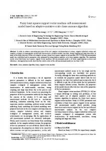
We consider models of order P = 2p with p pairs of conjugate complex poles on the unit disc and gain one. The excitation signal rt is white Gaussian noise with standard deviation σr = 0.3. A. Model Order Selection In Figure 2 the validation performance of an overparametrized model is shown as a function of the model order P . The two particular examples are generated for f1 and show that a model order can be selected based on the validation performance. Yet it is not necessarily the case that the true model order is revealed. From our simple experiments it seems that the model order tends to be under estimated. B. Correlation of Estimated Parameters with True Noise Model ˆ LS as an estimate for ak . Solving (D-3) we obtain a Projecting the model as described in Section III-C yields a ˆ SVD . To assess second estimate for ak which we denote as a the quality of the overparametrized model we investigate several quantities ˆ SVD ), 1) angle between estimates ^(ˆ aLS , a 1 http://www.scipy.org

0.4

2

4 6 simulated model order P

8

RMSE on validation set

(a) true model order P = 4

IV. N UMERICAL E XPERIMENTS All simulations are implemented in Python using Numpy1 . The RBF kernel is used for all considered models. Model selection is performed using an independent validation set. The regularization parameter γ and the kernel bandwidth σ are selected using grid search. Performance measures are reported on independent test sets in both cases. For the synthetic examples we compare the nonlinear systems given in [4]. 1) yt = f1 (ut ) = 0.2(1 − 6ut + 36u2t − 53u3t + 22u5t ) + et with ut uniformly distributed on [−0.5, 1.3] and 2) yt = f2 (yt−1 ) = sinc(yt−1 ) + et . The noise term et is generated with a linear AR(P) noise model according to

OVER-LS-SVM LS-SVM AR(P)-LS-SVM

0.6

0.6 OVER-LS-SVM LS-SVM AR(P)-LS-SVM

0.5

0.4

0.3

2

4 6 simulated model order P

8

(b) true model order P = 8 Fig. 2: Validation performance as a function of the noise model order P . Tested for f1 . The solid line is the validation performance of an overparametrized model of order P . The dashed line gives the performance of an AR(P)-LS-SVM model with the true noise model while the dotted line indicates the performance of a standard LS-SVM model.

2) angle between true parameters and plane spanned by ˆ SVD ]) and estimates ^(a, [ˆ aLS , a 3) individual angles between true parameters and estiˆ LS ), ^(a, a ˆ SVD ). mates ^(a, a 50 Monte Carlo simulations with different realizations of the noise model for orders P = 4 and P = 8 are shown Figures 3 and 4. The former depicts results for f1 while the latter shows results obtained with f2 . Especially for the lower order models the correlation of the different quantities are mostly below 10 degrees. Even for a model order of P = 8 for a lot of runs the correlations are still in a meaningful range. It seems that with the overparametrized formulation, the true noise model coefficients cannot be recovered. Yet the approximation is good enough to obtain predictive models that significantly outperform standard LS-SVM as shown in the next section. C. Performance of Projected Models We consider the same experiments as in the previous section but now compare prediction performances of 1) 2) 3) 4)

standard LS-SVM without noise model, AR(P)-LS-SVM given the true noise model (AR(P)), overparametrized LS-SVM (OVER, Alg. 1), ˆ LS estimates (DIRECT, AR(P)-LS-SVM with a Alg. 2), ˆ SVD estimates (SVD, Alg. 3). 5) AR(P)-LS-SVM with a

80

RMSE on test set

angle between estimate and true parameter

0.6

60 40 20

0.5

0.4

0.3

0

LS-SVM ˆ LS a

ˆ SVD a

AR(P)

ˆ SVD ] ^(ˆ ˆ SVD ) [ˆ aLS , a aLS , a

OVER

DIRECT

SVD

LS-SVM variant

estimate

(a) nonlinearity f1

(a) true model order P = 4

RMSE on test set

angle between estimate and true parameter

1.2

50

1 0.8 0.6 0.4 0.2

0 ˆ LS a

ˆ SVD a

LS-SVM

ˆ SVD ] ^(ˆ ˆ SVD ) [ˆ aLS , a aLS , a

ˆ LS Fig. 3: Correlation of true noise model parameters a with estimates a ˆ SVD based on 50 Monte Carlo simulations for f1 . and a

angle between estimate and true parameter

DIRECT

SVD

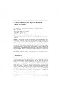
(b) nonlinearity f2 Fig. 5: Performance of different model structures (cf. Sec. IV-C) evaluated for different nonlinearities in 50 Monte Carlo runs. The true noise model order is P = 8.

Results for Monte Carlo simulations are shown in Figures 5.

40 30 20 10 0 ˆ LS a

ˆ SVD a

ˆ SVD ] ^(ˆ ˆ SVD ) [ˆ aLS , a aLS , a estimate

(a) true model order P = 4

angle between estimate and true parameter

OVER

LS-SVM variant

estimate (b) true model order P = 8

AR(P)

We can observe that the AR(P)-LS-SVM significantly outperforms standard LS-SVMs in a lot of cases. The overparametrized model is much better than LS-SVMs but does not perform as well as AR(P)-LS-SVM with the true parameters. For the projected model we observe that the estimate obtained by (D-3) is much more reliable than the obtained by the rank one approximation. In most cases the projected model slightly outperforms the overparametrized model. D. Projection Quality For the models evaluated in the previous sections, we can also analyse the quality of the projection step. Asqa measure PP 2 to asses how close W is to rank-1 we propose s0 / k=0 sk the ratio of the largest singular value over the energy in all singular values. Thus a value close to one in figure 6 corresponds to a matrix that is close to rank one. We can conclude that most of the energy is successfully concentrated in the largest singular value.

60 40 20 0 ˆ LS a

ˆ SVD a

ˆ SVD ] ^(ˆ ˆ SVD ) [ˆ aLS , a aLS , a estimate

(b) true model order P = 8 ˆ LS Fig. 4: Correlation of true noise model parameters a with estimates a ˆ SVD based on 50 Monte Carlo simulations for f2 . and a

E. Real Data We consider the second data set from the ESTSP08 benchmark [17]. The data set has one variable and contains 1300 hourly measurements of internet traffic in an academic network. We train a standard LS-SVM model with xt = [yt−1 , . . . , yt−m ]T for m = 1, . . . , 30 and select m = 17 as

s0 /

qP P

2 k=0 sk

1 0.8 0.6 0.4 f2 , P = 4

f2 , P = 8

f1 , P = 4

f1 , P = 8

experiment Fig. 6: Quality measure for the rank of W . Values close to one indicate a solution dominated by the largest singular value. Results are given for both nonlinear models and different noise model orders and compared for 50 Monte Carlo simulations.

TABLE I: Test performance for ESTSP08 [17] data set 2. model order P

RMSE on test set

0 (LS-SVM) 6 8 10 12 14

0.2195 0.2156 0.2103 0.2095 0.2073 0.1992

the order with the smallest validation error. Table I compares the performance on the last 10% of the data. These have not been used for estimating or selecting the model. It can be seen that the performance on this independent test set can be improved by considering a noise model. An open problem that requires further work is model order selection for the noise model. In [18] cross-validation is considered for the case of correlated errors. [19] uses auto- and crosscorrelations to select candidate noise models. The latter approach is more likely to lead to sparse models. V. C ONCLUSIONS We showed how to integrate a noise model with LSSVM based models and that doing so is beneficial in the presence of colored noise. For the case that the noise model is not known apriori we proposed a novel convex relaxation based on overparametrization to solve the otherwise nonconvex problem. This makes it viable to identify high order noise models without a significant increase in computational complexity. The identified coefficients of the noise model clearly deviate from the true parameters. Nevertheless the prediction capability of the identified models is superior to standard LS-SVM and can. in some cases, come close to the performance of a model given the true noise model parameters. Finally we demonstrated the applicability on two real world data sets. ACKNOWLEDGEMENTS Research supported by Research Council KUL: GOA AMBioRICS, GOA MaNet, CoE EF/05/006 Optimization in Engineering (OPTEC), IOF-SCORES4CHEM, several PhD/postdoc & fellow grants; Flemish Government: FWO: PhD/postdoc grants, projects G.0452.04 (new quantum algorithms), G.0499.04 (Statistics), G.0211.05 (Nonlinear), G.0226.06

(cooperative systems and optimization), G.0321.06 (Tensors), G.0302.07 (SVM/Kernel), G.0320.08 (convex MPC), G.0558.08 (Robust MHE), G.0557.08 (Glycemia2), G.0588.09 (Brain-machine); research communities (ICCoS, ANMMM, MLDM); G.0377.09 (Mechatronics MPC); IWT: PhD Grants, McKnow-E, Eureka-Flite+, SBO LeCoPro, SBO Climaqs, POM; Belgian Federal Science Policy Office: IUAP P6/04 (DYSCO, Dynamical systems, control and optimization, 2007-2011); EU: ERNSI; FP7-HD-MPC (INFSO-ICT-223854), COST intelliCIS, EMBOCOM; Contract Research: AMINAL; Other: Helmholtz: viCERP, ACCM, Bauknecht, Hoerbiger. Johan Suykens is a professor and Bart De Moor is a full professor at the Katholieke Universiteit Leuven, Belgium.

R EFERENCES [1] L. Ljung, System identification: Theory for the User. Prentice Hall PTR Upper Saddle River, NJ, USA, 1999. [2] A. Juditsky, H. Hjalmarsson, A. Benveniste, B. Delyon, L. Ljung, J. Sjoberg, and Q. Zhang, “Nonlinear black-box models in system identification: Mathematical foundations,” Automatica, vol. 31, pp. 1725–1750, December 1995. [3] J. Sjoberg, Q. Zhang, L. Ljung, A. Benveniste, B. Delyon, P.-Y. Glorennec, H. Hjalmarsson, and A. Juditsky, “Nonlinear black-box modeling in system identification: a unified overview,” Automatica, vol. 31, pp. 1691–1724, December 1995. [4] M. Espinoza, J. A. K. Suykens, and B. De Moor, “LS-SVM Regression with Autocorrelated Errors,” in Proc. of the 14th IFAC Symposium on System Identification (SYSID), Newcastle, Australia, March 2005, pp. 582–587. [5] V. N. Vapnik, Statistical Learning Theory. John Wiley & Sons, 1998. [6] B. Sch¨olkopf and A. J. Smola, Learning with Kernels. MIT Press Cambridge, Mass, 2002. [7] G. Wahba, Spline Models for Observational Data. SIAM, 1990. [8] C. E. Rasmussen and C. K. I. Williams, Gaussian processes for machine learning. Springer, 2006. [9] J. A. K. Suykens, T. Van Gestel, J. De Brabanter, B. De Moor, and J. Vandewalle, Least Squares Support Vector Machines. World Scientific, 2002. [10] J. A. K. Suykens, J. De Brabanter, L. Lukas, and J. Vandewalle, “Weighted least squares support vector machines: robustness and sparse approximation,” Neurocomputing, vol. 48, no. 1-4, pp. 85–105, 2002. [11] F. H. I. Chang and R. Luus, “A noniterative method for identification using Hammerstein model,” IEEE Transactions on Automatic Control, vol. 16, no. 5, pp. 464–468, 1971. [12] E.-W. Bai, “An optimal two-stage identification algorithm for Hammerstein-Wiener nonlinear systems,” Automatica, vol. 34, no. 3, pp. 333–338, 1998. [13] I. Goethals, K. Pelckmans, J. A. K. Suykens, and B. De Moor, “Subspace identification of Hammerstein systems using least squares support vector machines,” IEEE Transactions on Automatic Control, vol. 50, pp. 1509–1519, October 2005. [14] T. Falck, K. Pelckmans, J. A. K. Suykens, and B. De Moor, “Identification of Wiener-Hammerstein Systems using LS-SVMs,” in Proceedings of the 15th IFAC Symposium on System Identification (SYSID 2009), Saint-Malo, France, 2009, pp. 820–825. [15] D. J. C. MacKay, “Comparison of approximate methods for handling hyperparameters,” Neural Computation, vol. 11, pp. 1035–1068, 1999. [16] S. P. Boyd and L. Vandenberghe, Convex Optimization. Cambridge University Press, 2004. [17] A. Lendasse, T. Honkela, and O. Simula, “European symposium on time series prediction,” Neurocomputing, to appear, 2010. [18] K. De Brabanter, J. De Brabanter, J. A. K. Suykens, and B. De Moor, “Kernel Regression with Correlated Errors,” in Proceedings of the 11th Symposium on Computer Applications in Biotechnology, Leuven, Belgium, 2010. [19] M. Espinoza, J. A. K. Suykens, R. Belmans, and B. De Moor, “Electric Load Forecasting - Using kernel based modeling for nonlinear system identification,” IEEE Control Systems Magazine, vol. 27, pp. 43–57, 2007.