Linear Regression - Courses

Thought leaders in data science and analytics:

Linear Regression James G. Shanahan1 1Independent Consultant EMAIL: James_DOT_Shanahan_AT_gmail_DOT_com I 296A UC Berkeley Lecture 3 , Wednesday February 1, 2012 Berkeley I 296 A Data Science and Analytics Thought Leaders© 2011 James G. Shanahan

James.Shanahan_AT_gmail.com

1

• 

General Course References (Advanced) R

–  Practical Regression and Anova using R, http://cran.r-project.org/doc/contrib/Faraway-PRA.pdf ,by JJ Faraway (please download PDF) –  John Fox (2010), Sage, An R and S-PLUS Companion to Applied Regression (second edition, PDFs) •  Preface to the book, Chapter 1 - Getting Started With R (PDFs available) •  Chapter 6 - Diagnosing Problems in Linear and Generalized Linear Models –  The R book, by Michael J. Crawley, Wiley 2009

• 

Linear Regression –  Analyzing Multivariate Data by James Lattin, J. Douglas Carroll, Paul E. Green. Thompson 2003.ISBN: 0-534-349749 –  Introduction to Linear Regression Analysis. D. Montgomery, E. Peck. GG Vining (4th Edition)

• 

Data mining –  TSK Introduction to Data Mining, Pang-ning Tan, Michael Steinbach, Vipin Kumar. Addison Wesley 2005. ISBN: 0-321-32136-7

• 

Machine Learning, probability theory –  Duda, Hart, & Stork (2000). Pattern Classification. http://rii.ricoh.com/~stork/DHS.html –  Modern Multivariate Statistical Techniques: Regression, Classification, and manifold Learning, Alan Julian Izenman, Springer, 2008, ISBN 978-0-387-78188-4 –  Pattern Recognition and Machine Learning, Christopher M. Bishop, Springer –  Elements of Machine Learning, Friedman et al., 2009, Download from here http://www-stat.stanford.edu/~tibs/ElemStatLearn/download.html

• 

General AI –  Artificial Intelligence: A Modern Approach (Third edition) by Stuart Russell and Peter Norvig.

Berkeley I 296 A Data Science and Analytics Thought Leaders© 2011 James G. Shanahan


2

Lecture Outline •  Linear Regression: a brief intro •  A quick statistics review –  Mean, expected value, variance, stdev, quantiles, stats in R

•  Locally Weighted Linear Regression •  Exploratory Data Analysis •  Simple Linear Regression –  Normal Equations –  Closed form Solution –  Variance of the estimators

•  Good model?



3

Regression and Model Building •  Regression analysis is a statistical technique for investigating and modeling the relationship between variables. –  Assume two variables, x and y. Model relationship as y~x (aka y =f (x)) as a linear relationship •  y=β0 + β1x –  Not a perfect fit generally; Account for difference between model prediction and the actual target value as a statistical error ε •  y=β0 + β1x + ε #This is a linear regression model –  This error ε maybe made up of the effects of other variables, measurement errors and so forth –  Customarily x is called the independent variable (aka predictor or regressor) and y the dependent variable (aka response variable) –  Simple linear regression involves only one regressor variable –  Suppose we can fix the value of x and observe the corresponding value of the response y. Now if x is fixed, the random component ε determines the properties of y Berkeley I 296 A Data Science and Analytics Thought Leaders© 2011 James G. Shanahan


4

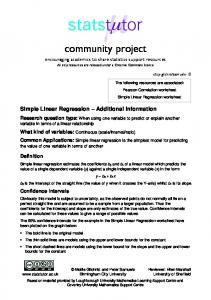
Simple Linear Regression Model Y

Regression Plot

µy|x=α + β x y

Error: ε

} β = Slope

}

{

1

{

Actual observed values of Y (y) differ from the expected value (µy|x ) by an unexplained or random error(ε):

α = Intercept

0

The simple linear regression model posits an exact linear relationship between the expected or a v e r a g e v a l u e o f Y, t h e dependent variable Y, and X, the independent or predictor variable: µy|x= α+β x

X

x

Berkeley I 296 A Data Science and Analytics Thought Leaders©

y = µy|x + ε =α +β x + ε 2011 James G. Shanahan James.Shanahan_AT_gmail.com

5

ε determines the properties of the response y •  Suppose we can fix the value of x and observe the corresponding value of the response y. Now if x is fixed, the random component ε determines the properties of y. •  Suppose the mean and variance of ε are 0 and σ2, respectively. Then the mean response at any value of the regressor variable (x) is •  E(y|x) = µy|x=E(β0 + β1 x + ε) = β0 + β1 x •  The variance of y given any value x is •  Var(y|x) = σy|x2 = Var(β0 + β1 x + ε) = σ2 –  The variability of y at a particular value of x is determined by the variance of the error component of the model σ2. This implies that there is a distribution of y values at each x and the variance of this distribution is the same at each x 2 implies the observed values y will fall close to the line. –  Small σ Berkeley I 296 A Data Science and Analytics Thought Leaders© 2011 James G. Shanahan James.Shanahan_AT_gmail.com

6

Assumptions of the Simple Linear Regression Model •  • 

• 

The relationship between X and Y is a straight-Line (linear) relationship. The values of the independent variable X are assumed fixed (not random); the only randomness in the values of Y comes from the error term ε. The errors ε are uncorrelated (i.e. Independent) in successive observations. The errors ε are Normally distributed with mean 0 and variance σ2(Equal variance). That is: ε~ N(0,σ2)

Y

LINE assumptions of the Simple Linear Regression Model

µy|x=α + β x

y Identical normal distributions of errors, all centered on the regression line.

y~N(µy|x, σy|x2) x



X 7

Example •  Let y be a student s college achievement, measured by his/her GPA. This might be a function of several variables: –  –  –  – 

x1 = x2 = x3 = x4 =

rank in high school class high school’s overall rating high school GPA SAT scores

•  We want to predict y using knowledge of x1, x2, x3 and x4.



8

Some Questions •  Which of the independent variables are useful and which are not? •  How could we create a prediction equation to allow us to predict y using knowledge of x1, x2, x3 etc? •  How good is this prediction?

We start with the simplest case, in which the response y is a function of a single independent variable, x. Berkeley I 296 A Data Science and Analytics Thought Leaders© 2011 James G. Shanahan


9

A Simple Linear Model •  We use the equation of a line to describe the relationship between y and x for a sample of n pairs, (x, y). •  If we want to describe the relationship between y and x for the whole population, there are two models we can choose

• Deterministic Model: y = β0 + β1 x • Probabilistic Model: – y = deterministic model + random error – y = β0 + β1 x + ε Berkeley I 296 A Data Science and Analytics Thought Leaders© 2011 James G. Shanahan


10

A Simple Linear Model •  Since the measurements that we observe do not generally fall exactly on a straight line, we choose to use: •  Probabilistic Model: –  y = β0 + β1x + ε

–  E(y) = β0 + β1x

Points deviate from the line of means by an amount ε where ε has a normal distribution with mean 0 and variance σ2.



11

The Random Error p The line of means, E(y) = α + βx , describes average value of y for any fixed value of x. p The population of measurements is generated as y deviates from the population line by ε. We estimate α

and β using sample information.



12

Linear Regression App •  http://www.duxbury.com/ authors/mcclellandg/tiein/ johnson/reg.htm •  Play with App to see the relationship between R^2 and the error



13

Simple Linear Regression in R

180

http://www-stat.stanford.edu/~jtaylo/courses/stats203/R/ introduction/introduction.R.html heights.table