Local Polynomial Regression Estimators in Survey ... - Semantic Scholar

Local Polynomial Regression Estimators in Survey Sampling

F. Jay Breidt and Jean D. Opsomer Iowa State University June 8, 2000

Abstract

Estimation of nite population totals in the presence of auxiliary information is considered. A class of estimators based on local polynomial regression is proposed. Like generalized regression estimators, these estimators are weighted linear combinations of study variables, in which the weights are calibrated to known control totals, but the assumptions on the superpopulation model are considerably weaker. The estimators are shown to be asymptotically design-unbiased and consistent under mild assumptions. A variance approximation based on Taylor linearization is suggested and shown to be consistent for the design mean squared error of the estimators. The estimators are robust in the sense of asymptotically attaining the Godambe-Joshi lower bound to the anticipated variance. Simulation experiments indicate that the estimators are more ecient than regression estimators when the model regression function is incorrectly speci ed, while being approximately as ecient when the parametric speci cation is correct. AMS 2000 subject classi cation. Primary 62D05; secondary 62G08. Key words and phrases. Calibration, generalized regression estimation, Godambe-Joshi lower bound, model-assisted estimation, nonparametric regression. Iowa State University of Science and Technology, Statistical Laboratory and Department of Statistics, 221 Snedecor Hall, Ames, IA 50011{1210.

Local Survey Regression Estimators

1

1 Introduction 1.1 Background

In many survey problems, auxiliary information is available for all elements of the population of interest. Population registers in some countries contain age and taxable income for all residents. Studies of labor force characteristics or household expenditure patterns might bene t from these auxiliary data. Geographic information systems may contain measurements derived from satellite imagery for all locations. These spatially-explicit data can be useful in augmenting measurements obtained in agricultural surveys or natural resource inventories. Indeed, use of auxiliary information in estimating parameters of a nite population of study variables is a central problem in surveys. One approach to this problem is the superpopulation approach, in which a working model describing the relationship between the auxiliary variable x and the study variable y is assumed. Estimators are sought which have good eciency if the model is true, but maintain desirable properties like asymptotic design unbiasedness (unbiasedness over repeated sampling from the nite population) and design consistency if the model is false. Typically, the assumed models are linear models, leading to the familiar ratio and regression estimators (e.g., Cochran, 1977), the best linear unbiased estimators (Brewer, 1963; Royall, 1970), the generalized regression estimators (Cassel, Sarndal, and Wretman, 1977; Sarndal, 1980; Robinson and Sarndal, 1983), and related estimators (Wright, 1983; Isaki and Fuller, 1982). The papers cited vary in their emphasis on design and model, but it is fair to say that all are concerned to some extent with behavior of the estimators under model misspeci cation. Given this concern with robustness, it is natural to consider a nonparametric class of models for , because they allow the models to be correctly speci ed for much larger classes of functions. Kuo (1988), Dorfman (1992), Dorfman and Hall (1993), and Chambers, Dorfman, and Wehrly (1993) have adopted this approach in constructing model-based estimators. This paper describes theoretical properties of a new type of model-assisted nonparametric regression estimator for the nite population total, based on local polynomial smoothing. Local polynomial regression is a generalization of kernel regression. Cleveland (1979) and Cleveland and Devlin (1988) showed that these techniques are applicable to a wide range of problems. Theoretical work by Fan (1992, 1993) and Ruppert and Wand (1994) showed that it has many desirable theoretical properties, including adaptation to the design of the covariate(s), consistency and asymptotic unbiasedness. Wand and Jones (1995) provide a clear explanation of the asymptotic theory for kernel regression and local polynomial regression. The monograph by Fan and Gijbels (1996) explores a wide range of application areas of local polynomial regression techniques. However, the application of these techniques to model-assisted survey sampling is new. In Section 1.2 we introduce the local polynomial regression estimator and in Section 1.3 we state assumptions used in the theoretical derivations of Section 2, in which our main results are described. Section 2.1 shows that the estimator is a weighted linear combination of study variables in which the weights are calibrated to known control totals. Section 2.2 contains a proof that the estimator is asymptotically design unbiased and design consistent, and Section 2.3 provides an approximation to its mean squared error and a consistent estimator of the mean squared error. Section 2.4 provides sucient conditions for asymp-


2

totic normality of the local polynomial regression estimator and establishes a central limit theorem in the case of simple random sampling. We show that the estimator is robust in the sense of asymptotically attaining the Godambe-Joshi lower bound to the anticipated variance in Section 2.5, a result previously known only for the parametric case. Section 3 reports on a simulation study of the design properties of the estimator, which is competitive with the classical survey regression estimator when the population regression function is linear, but dominates the regression estimator when the regression function is not linear. Our estimator also performs well relative to other parametric and nonparametric estimators, both model-assisted and model-based.

1.2 Proposed Estimator

Consider a nite population UN = f1; : : :; i; : : :; N g. For each i 2 UN , an auxiliary variable xi is observed. In this article, we explore the case in which the xi are scalars. But it will be

clear from the de nition of the estimator later in this section that there is no inherent reason to do so, except to make the theory more tractable. Most of the properties of the estimator we will discuss are also expected to hold for multi-dimensional xi , though the \curse of dimensionality" implies that practical applications would be complicated by sparseness of the regressors in the design space. Sparseness adjustments (e.g. Hall and Turlach, 1997) or dimension-reducing alternatives such as additive modeling (Hastie and Tibshirani, 1990) would then need P to be employed. These topics will be explored elsewhere. Let tx = i2UN xi . A probability sample s is drawn from UN according to a xed-size sampling design pN (), where pN (s) is the probability the sample s. Let nN be P p (ofs)drawing the size of s . Assume = Pr f i 2 s g = > 0 and ijN = Pr fi; j 2 sg = iN s:i2s N P s:i;j 2s pN (s) > 0 for all i; j 2 UN . For compactness of notation we will suppress the subscript N and write i , ij in what follows. The study variable yi is observed for each i 2 s. The goal is to estimate ty = Pi2UN yi . Let Ii = 1 if i 2 s and Ii = 0 otherwise. Note that Ep [Ii ] = i , where Ep [] denotes expectation with respect to the sampling design (that is, averaging over all possible samples from the nite hpopulation). Using this notation, an estimator ty of ty is said to be designi unbiased if Ep ty = ty . A well-known design-unbiased estimator of ty is the HorvitzThompson estimator, X X yiIi t^y = yi = (1) i2s i

i2UN

i

(Horvitz and Thompson, 1952). The variance of the Horvitz-Thompson estimator under the sampling design is X (2) (ij ? i j ) yi yj : Varp t^y = i;j 2UN

i j

Note that t^y does not depend on the fxi g. It is of interest to improve upon the eciency of the Horvitz-Thompson estimator by using the auxiliary information. The estimator we propose is motivated by modeling the nite population of yi 's, conditioned on the auxiliary variable xi , as a realization from an in nite superpopulation, , in which yi = m(xi ) + "i


3

where "i are independent random variables with mean zero and variance v (xi ), m(x) is a smooth function of x, and v (x) is smooth and strictly positive. Given xi , m(xi) = E [yi ] and so is called the regression function, while v (xi) = Var (yi ) and so is called the variance function. Let K denote a continuous kernel function and let hN denote the bandwidth. We begin by de ning the local polynomial kernel estimator of degree q based on the entire nite population. Let yU = [yi ]i2UN be the N -vector of yi 's in the nite population. De ne the N (q + 1) matrix 2 1 x1 ? xi (x1 ? xi)q 3 75 = h 1 xj ? xi (xj ? xi)q i ; .. X Ui = 64 ... ... . j 2UN 1 xN ? xi (xN ? xi )q and de ne the N N matrix 1 xj ? xi : W = diag K Ui

hN hN j 2UN Let er represent a vector with a 1 in the rth position and 0 elsewhere. Its dimension will

be clear from the context. The local polynomial kernel estimator of the regression function at xi , based on the entire nite population, is then given by ? mi = e01 X 0Ui W UiX Ui ?1 X 0UiW Ui yU = w0Ui yU ; (3) which is well-de ned as long as X 0Ui W UiX Ui is invertible. If these mi 's were known, then a design-unbiased estimator of ty would be the generalized dierence estimator X X mi (4) ty = yi ? mi + i2s

i

i2UN

(Sarndal, Swensson, and Wretman, 1992). The design variance of the estimator (4) is

X Varp ty = (ij ? i j ) yi ? mi yj ? mj ; i j i;j 2UN

(5)

which we would expect to be smaller than (2); the deviations fyi ? mi g = f(m(xi ) ? mi )+ i g will typically have smaller variation than the fyi g for any reasonable smoothing procedure under the model . The population estimator mi is the traditional local polynomial regression estimator for the unknown function m(), widely discussed in the nonparametric regression literature. In the present context, it cannot be calculated, because only the yi in s UN are known. Therefore, we will replace the mi by a sample-based consistent estimator. Let ys = [yi ]i2s be the nN -vector of yi 's obtained in the sample. De ne the nN (q + 1) matrix

X si = h 1

and de ne the nN nN matrix

i

xj ? xi (xj ? xi)q j2s ;

(

)

W si = diag j1hN K xjh?N xi

j 2s

:


4

A sample design-based estimator of mi is then given by

m^ oi = e01

?X 0 W si

X

si si

?

1

X0siW siys = wosi0 ys;

(6)

as long as X 0si W si X si is invertible. When we substitute the m ^ oi into (4), we have the local polynomial regression estimator for the population total o X X m^ o: (7) t~o = yi ? m^ i + y

i2s

i

i

i2UN

The sample estimator in (6) diers in one important way from the traditional local polynomial regression estimator. The presence of the inclusion probabilities in the \smoothing weights" wosi make our sample-based estimator m ^ i a design-consistent estimator of the nite population smooth mi , which is based on some (not necessarily optimal) bandwidth hN , considered xed here for any N . In real survey problems, hN will rarely be optimal because a single bandwidth would be chosen and used to compute weights to be applied to all study variables. Despite this, the topics of theoretically optimal and practical bandwidth selection are clearly of some interest, and will be addressed elsewhere. Regardless of the choice of hN , mi is a well-de ned parameter of the nite population. Speci cally, mi is a function of nite population totals, each of which can be estimated consistently by their corresponding Horvitz-Thompson estimators. That is, we have included probability weights in the smoothing weights in order to construct asymptotically design-unbiased and designconsistent estimators of the nite population smooths mi (not m(xi)). This is consistent with the development of the generalized regression estimator (GREG), which our procedure reverts to as the bandwidth becomes large. In principle, the estimator (6) can be unde ned for certain i 2 UN , even if the population estimator in (3) is de ned everywhere: if for some sample s, there are less than q + 1 observations in the support of the kernel at some xi , then the matrix X 0si W si X si will be singular. This is not a problem in practice, because it can be avoided by selecting a bandwidth that is suciently large to make X 0si W si X si invertible at all locations xi . However, that situation cannot be excluded theoretically as long as the bandwidth is considered xed for a given population. Therefore, for the purpose of the theoretical derivations in Section 2, we will consider an adjusted sample estimator that is guaranteed to exist for any sample s UN . The adjusted sample estimator for mi is given by

e X W siX si + diag

m^ i = 01

0 si

q ! ? +1

N2

j =1

1

X0siW siys = w0siys

(8)

for some small > 0. The terms N ?2 in the denominator are small order adjustments that ensure the estimator is well-de ned for all s UN . This adjustment was also used by Fan (1993) for the same reason when the xi are considered random. Another possible adjustment would consist of replacing the usual choice of a kernel with compact support by one with in nite support such as the Gaussian kernel. In practice, however, such kernels have been found to increase the computational complexity of local polynomial tting and result in less satisfactory ts compared to those obtained with compactly supported kernels.


5

The adjustment proposed here maintains the sparseness of the smoothing vector wsi , and its eect can be made arbitrarily small by choosing accordingly. We let X ^ i + X m^ ~t = yi ? m (9) y

i2s

i

i2UN

i

denote the local polynomial regression estimator that uses the adjusted sample smoother in (8). The remainder of this article will be concerned with studying the properties of t~y (and t~oy when appropriate). The development of the model-assisted local polynomial regression estimator above could clearly be followed for other kinds of smoothing procedures. We focus on the local polynomial methodology because it is of considerable practical interest. In the case q = 0, the estimator relies on kernel regression, and behaves like a classical poststrati cation estimator, but mixed over dierent possible stratum boundaries. As the bandwidth becomes large, P the estimator reverts to the Hajek estimator, N t^y =N^ , where N^ = s 1=k . In the local linear regression (q = 1) case, the estimator looks something like a poststrati ed regression estimator, and the estimator reverts to the classical regression estimator as the bandwidth becomes large.

1.3 Notation and Assumptions

Our basic approach to study the design and model properties of the estimators will be to use a Taylor linearization for the sample smoother m^ i . Note rst that we can write mi = f (N ?1 ti ; 0) and m^ i = f (N ?1^ti; ) for some function f , where the comes from the adjustment in equation (8) and vanishes in the population t (3),

ti = [tig ]Gg

2 xk ? xi 3G 2 X 3G X 1 y 5 =4 5 =4 zigk zigk h K h

h iG

2 xk ? xi Ik 3G 2 X Ik 3G X 1 y 5 = 4 zigk 5 K z =4 igk h h N N k k k2UN k2UN g g

=1

and

^ti = tîg

g=1

k2UN N

N

g=1

=1

k2UN

y . For local polynomial regression of degree q , for suitable zigk y as G1 = 2q + 1, we can write the zigk ( ? xi)g?1 g G1 y zigk = ((xxk ? g ? G ? 1 1 yk g > G 1 : k xi )

g=1

=1

G = 3q + 2. If we let

Examples: The kernel regression (q = 0) and local linear regression (q = 1) cases are of particular interest.

In the case q = 0, X 1 xk ? x i X 1 xk ? xi K K h and t = yk ; ti = i hN N k2UN hN k2UN hN 1

2


6

so that (3) is the Nadaraya-Watson estimator, based on the entire nite population, of the model regression function: mi = t?i11 ti2 . Ignoring the -adjustment, the corresponding sample-based estimator is then m^ 0i = t^?i11 tî2 :

In the case of local linear regression (q = 1), X 1 xk ? xi X 1 xk ? xi K h K h ; ti = (xk ? xi ); ti = N N k2UN hN k2UN hN X 1 xk ? xi X 1 xk ? xi K K h ( x ? x ) ; t = yk ; ti = k i i hN N k2UN hN k2UN hN X 1 xk ? xi and ti = K h (xk ? xi )yk : N k2UN hN 2

1

2

3

4

5

Then

mi = tit3 tit4 ??tit22ti5 ; i1 i3

i2

with the corresponding sample-based estimator ^^ ^^ m^ 0i = ti^3 ti^4 ? ti^22ti5 : ti1 ti3 ? ti2 Using a Taylor approximation, de ne

X Ik @ m^ i 1 RiN = m^ i ? mi ? N zik ? 1 ? @ k2UN

where

k

@ m^ i : zik = zigk ? 1 ^ g=1 @ (N tig ) tî =ti ;=0 G X

^ ti=ti;=0 N 2

(10)

To prove our theoretical results, we make the following assumptions. A1 Distribution of the errors under : the errors "i are independent and have mean zero, variance v (xi ), and compact support, uniformly for all N . A2 For each N , the xi are considered xed with respect to the Rsuperpopulation model x f (t)dt, where f () . The xi are independent and identically distributed F (x) = ?1 is a density with compact support [ax; bx] and f (x) > 0 for all x 2 [ax ; bx]. A3 Mean and variance functions m, v on [ax; bx]: the mean function m() is continuous and has q + 1 continuous derivatives, and the variance function v (x) is continuous and strictly positive.


7

A4 Kernel K : the kernel K () has compact support [?1; 1], is symmetric and continuous, and satis es Z u b q = cK (u) du = 6 0; 1

2 ( +1) 2

?1

where bac denotes the integer part of a.

A5 Sampling rate nN N ? and bandwidth hN : as N ! 1, nN N ? ! 2 (0; 1), hN ! 0 and NhN =(log log N ) ! 1. A6 Inclusion probabilities i and ij : for all N , mini2UN i > 0, mini;j 2UN ij > 0 and lim sup nN i;j 2max j ? ij j < 1: U i6 j ij 1

1

2

N !1

N: =

A7 Additional assumptions involving higher-order inclusion probabilities: lim n max Ep [(Ii ? i )(Ii ? i )(Ii ? i )(Ii ? i )] < 1; 2

N !1 N (i1 ;i2 ;i3 ;i4 )2D4;N

1

1

2

2

3

3

4

4

where Dt;N denotes the set of all distinct t-tuples (i1; i2; : : :; it) from UN ,

lim N !1 and

Ep [(Ii1 Ii2 ? i1i2 )(Ii3 Ii4 ? i3i4 )] = 0;

max

h i Ep (Ii1 ? i1 ) (Ii2 ? i2 )(Ii3 ? i3 ) < 1:

i ;i ;i ;i 2D4;N

( 1 2 3 4)

lim sup nN N !1

max

i ;i ;i 2D3;N

( 1 2 3)

2

Remarks:

1. The assumption of compactly supported errors in A1 is made to simplify bounding arguments used extensively in the proofs. It is possible to obtain the results using nite population moment assumptions of the form X k " < 1 with -probability one; lim sup 1 N !1

N i2UN

i

though this signi cantly complicates the arguments. 2. The fxi g are kept xed with respect to the model to make the results in later sections look like traditional (non-asymptotic) nite population results. The assumption A2, however, ensures that the fxi g are a random sample from a continuous distribution. In order to maintain the article's emphasis on the model and sampling design pN , the conditioning on the xi 's will be suppressed in what follows.


8

3. The assumption of compactly supported errors is used to establish uniform integrability needed to allow taking expectations through Taylor approximations. Alternatively, it is possible to modify A3 and A4 to include additional assumptions about smoothness of the rst derivatives of the various functions, which are normally not required for local polynomial regression. Assumption A5 would then also be modi ed by a factor of log log N= log N in the bandwidth rate. These adjustments, together with moment assumptions on the "k , would guarantee uniform convergence of the nonparametric regression components of the estimator. Such assumptions were used in Opsomer and Ruppert (1997) for the same purpose in the context of additive model tting. The assumptions are based on the uniform convergence results of Pollard (1984). 4. Assumption A6 is similar to assumptions used by Robinson and Sarndal (1983), who examined the parametric regression case. A7 extends those assumptions. Assumptions A6 and A7 involve rst through fourth-order inclusion probabilities of the design. These assumptions hold for simple random sampling without replacement. Let k denote the kth order inclusion probability of k distinct elements under simple random sampling without replacement. Then A6 is well-known, and it is easy to check that the rst expression in A7 becomes

N 2(4 ? 413 + 6212 ? 341) = O(1); the second one becomes

4 ? 22 = O(N ?1);

and the third expression becomes

nN (3 ? 212 + 31 ? 213 + 5212 ? 341) = O(1): 5. By similar arguments, A6 and A7 will hold for strati ed simple random sampling with xed stratum boundaries determined by the xi 's and for related designs. If clustering is a signi cant feature of the design, then there are at least two possibilities for auxiliary information: availability at the element level and availability at the cluster level. A6 and A7 will generally not hold (at the element level) for designs with nontrivial clustering. The rst case, however, is rare in practice because a clustered design is unlikely to be used when such detailed element-level frame information is available. In the second case, elements may be fully enumerated within selected clusters or they may be subsampled. If they are fully enumerated, the assumptions above apply directly to the sample of clusters with cluster-level auxiliary information. If they are subsampled, then the framework above would require extensions to describe the subsampling procedure. Though such extensions are beyond the scope of the present investigation, we believe that results similar to those described below would continue to hold under reasonable assumptions. These remarks indicate that it should be possible to obtain the results we describe under a variety of asymptotic formulations. The speci c assumptions we describe are only one possibility, though we believe they are reasonable and they give some insight into when the asymptotic approximations we describe would be expected to work.


9

2 Main Results

2.1 Weighting and Calibration

Note from (7) that

~toy

=

X yi

X

+ i2s i j 2UN

1 ? Ij j

!

wosj0 ys

9 8 ! X< 1 X Ij wo0 e = y 1 ? + = j sj i; i i2s : i j 2UN X =

i2s

!is yi :

(11)

Thus t~oy is a linear combination of the sample yi 's, where the weights are the inverse inclusion probabilities, suitably modi ed to re ect the information in the auxiliary variable xi . The same reasoning applies directly to t~y . Because the weights are independent of yi , they can be applied to any study variable of interest. In particular, they can be applied to the auxiliary variables 1; xi; : : :; xqi . Then it is straightforward to verify that for the local polynomial regression estimator t~oy , X ` X ` !is xi = xi i2s

i2UN

for ` = 0; 1; : : :; q . That is, the weights are exactly calibrated to the q + 1 known control totals N; tx ; : : :; txq . Calibration is a highly desirable property for survey weights, and in fact motivates the class of estimators considered by Deville and Sarndal (1992). Part of the desirability of the calibration property comes from the fact that if m(xi) is exactly a q th degree polynomial function of xi , then t~oy is exactly model-unbiased. In addition, the control totals are often published in ocial tables or otherwise widely disseminated as benchmark values, so reproducing them from the sample is reassuring to the user. While the local polynomial regression estimator t~y is no longer exactly calibrated, it remains approximately so, in the sense that its weights reproduce the control totals to terms of o(N ?1 ). We omit the proof.

2.2 Asymptotic Design Unbiasedness and Consistency

The price for using m^ i 's in place of mi 's in the generalized dierence estimator (4) is design bias. The estimator t~y is, however, asymptotically design unbiased and design consistent under mild conditions, as the following theorem demonstrates: Theorem 1 Assume A1{A7. Then the local polynomial regression estimator X t~y = (yi ? m^ i ) Ii + m^ i i2UN

i

is asymptotically design unbiased (ADU) in the sense that # "~ t ? t y y = 0 with -probability one; lim E N !1 p

N

Local Survey Regression Estimators and is design consistent in the sense that

h

10

i

= 0 with -probability one lim E I N !1 p fj~ty?ty j>Ng for all > 0.

The proof of this and following theorems rely on several technical lemmas which are gathered in the Appendix. Proof of Theorem 1: By Markov's inequality, it suces to show that t~y ? ty lim E N = 0: p N !1 Write Then

t~y ? ty = X yi ? mi Ii ? 1 + X m^ i ? mi 1 ? Ii : N i N i i2UN N i2UN

X yi ? mi Ii ~ ? ty E ?1 Ep ty N p N i i2UN

8 2 < X (m^ i ? mi) 3 2 X (1 ? i? Ii) 5 Ep 4 + :Ep 4 N N i2UN i2UN 1

2

2

39 == 5; : 1 2

(12)

Under A1{A6 and using the fact that

X (yi ? mi )2 < 1 lim sup N1 N !1

i2UN

by Lemma 2(iv), the rst term on the right of (12) converges to zero as N ! 1, following the argument of Theorem 1 in Robinson and Sarndal (1983). Under A6,

2 3 ? Ii ) X (1 ? i 5 = X i(1 ? i) 1 : Ep 4 N i2UN i2UN Ni 1

2

2

Combining this with Lemma 4, the second term on the right of (12) converges to zero as

N ! 1, and the theorem follows.

2.3 Asymptotic Mean Squared Error

In this section we derive an asymptotic approximation to the mean squared error of the local polynomial regression estimator and propose a consistent variance estimator. We rst show that the asymptotic mean squared error of the local polynomial regression estimator is equivalent to the variance of the generalized dierence estimator, given in (5).


11

Theorem 2 Assume A1{A7. Then ! ~y ? ty nN X (y ? m )(y ? m ) ij ? ij + o(1): t =N nN E p N i i j j 2

2

i j

i;j 2UN

(13)

Proof of Theorem 2: Let

aN = n1N=2 Then

X yi ? mi Ii ^ i Ii ? 1 : = X mi ? m ? 1 and b = n N N i N i i2UN i2UN N

h i

Ep a2N

1 2

nN X (y ? m )(y ? m ) ij ? i j = N i i j j 2 i j

i;j 2U

1 nNNmaxi;j2U i6 j jij ? ij j X (yi ? mi) N + N ; i2UN so that lim supN !1 Ep aN < 1 by A6. By Lemma 5, Ep bN = o(1), so that h i h i = = o(1): Ep [aN bN ] Ep aN Ep bN 2

: = 2

2

2

2

Hence,

2

1 2

2 !3 h i h i h i ~ t ? t nN Ep 4 y y 5 = Ep aN + 2Ep [aN bN ] + Ep bN = Ep aN + o(1); 2

N

2

2

2

and the result is proved. The next result shows that the asymptotic mean squared error in (13) can be estimated consistently under mild assumptions.

Theorem 3 Assume A1{A7. Then ? ? lim n E V^ (N ~ty ) ? AMSE(N t~y ) = 0; N !1 N p 1

where and

V^ (N ?1 ~ty ) = N12 AMSE(N ?1 ~ty ) =

X i;j 2UN

1

(yi ? m ^ i )(yj ? m^ j ) ij ?i j Ii Ij i j

ij

(14)

1 X (y ? m )(y ? m ) ij ? i j : i i j j N2 i j i;j 2UN

Therefore, V^ (N ?1 ~ty ) is asymptotically design unbiased and design consistent for AMSE(N ?1t~y ).


12

Proof of Theorem 3: Write X (yi ? mi )(yj ? mj ) ij ? i j Ii Ij ? ij : AN = nN Ep 12

N

i j

i;j 2UN

ij

Now

1 0 X I I ? ? 1 (yi ? mi )(yj ? mj ) ij i j i j ij A nN E p @ N 2

2

= n2N

i j

i;j 2UN

2

ij

X 1 ? i 1 ? k (yi ? mi) (yk ? mk ) ik ? ik 2

N4 i k X X 1 ? i k` ? k ` (yi ? mi)2(yk ? mk )(y` ? m`) +2n2N k ` N4 i2UN k;`2UN :k6=` i Ii ? i I I ? Ep k ` k` i k` X X ij ? ij k` ? k ` (yi ? mi)(yj ? mj )(yk ? mk )(y` ? m` ) +n2N k ` N4 i;j 2UN :i6=j k;`2UN :k6=` i j # " I I ? I I ? k ` k` i j ij Ep k` ij = a1N + a2N + a3N : i;k2UN

i

2

But

a1N n2N

k

X (yi ? mi) N + nN 4

i2UN

1 N + 3

3

2

X

4

i;k2UN :i6=k nN maxi;k2UN :i6=k jik ? i k j

N4

which goes to zero as N ! 1, and 2 a (nN maxi;k2UN :i6=k jik ? ik j) N

3

(yi ? mi )2(yk ? mk )2 jik ? i k j

X

4 N 4 X (yi ? mi)4 N i2UN

42

X

j(yi ? mi)(yj ? mj )(yk ? mk )(y` ? m`)j N i;j2U"N i6 j k;`2UN k6 ` # Ep IiIj? ij Ik I`? k` ij k` O(N ? ) + (nN maxi;k2UN i6 k jik ? ik j) " # X I I ? I I ? (yi ? mi ) ; i j ij k ` k` E i;j;k;`max p i2UN N ij k` 2D4;N which converges to zero as N ! 1 by A7. The Cauchy-Schwarz inequality may then be applied to show that a N ! 0 as N ! 1, and it follows that AN ! 0 as N ! 1.

: =

4

: =

: = 4 2

1

2

4

(

2

)


13

Next, write X BN = nN Ep N12 f2(yi ? mi)(mj ? m^ j ) + (mi ? m^ i)(mj ? m^ j )g ij ?ij IiIj i;j 2UN

i j

(P

ij

) P 2nN maxi;j2U i6 j jij ? ij j 2nN (yi ? mi ) i2UN Ep (mi ? m^ i ) = i 2 U N N +N N N nN maxi;j2U i6 j jij ? ij j nN P Ep (mi ? m^ i) i2UN N + + : =

2

2

2

2

2

: =

2

2 N

N ! 0 as N ! 1 using A6 and Lemma 4. The result then follows because nN Ep jV^ (N ? ~ty ) ? AMSE(N ? t~y )j AN + BN : 1

1

An alternative variance estimator could be constructed by replacing the term i?1j?1 in (14) with the product of weights !is !js from (11). This is the analogue of the weighted residual technique (Sarndal, Swensson, and Wretman, 1989) for estimating the variance of the general regression estimator, which they propose to improve the conditional and small sample properties of the variance estimator. Simpli ed versions of (13) and (14) are given in Corollary 1 below for the case of simple random sampling.

2.4 Asymptotic Normality

The local polynomial regression estimator inherits the limiting distributional properties of the generalized dierence estimator, as we now demonstrate.

Theorem 4 Assume that A1{A7 hold and let ty and Varp ty be as de ned in (4) and (5), respectively. Then,

N ?1(ty ? ty ) L ! N (0; 1) Var1p=2(N ?1ty )

as N ! 1 implies

N ?1(t~y ? ty ) ! L ^V 1=2(N ?1t~y ) N (0; 1)

as N ! 1, where V^ (N ?1t~y ) is given in (14).

Proof of Theorem 4: From the proof of Theorem 2,

N ?1 (t~y ? ty ) =

X yi ? mi Ii ? 1 + o (n? = ) = N ? (t ? t ) + o (n? = ):

i2UN

N

i

p N

1 2

1

y

y

p N

1 2

Further, V^ (N ?1 ~ty )=AMSE(N ?1t~y ) !p 1 by Theorem 3, so the result is established.

1 2


14

Thus, establishing a central limit theorem (CLT) for the local polynomial regression estimator is equivalent to establishing a CLT for the generalized dierence estimator, which in turn is essentially the same problem as establishing a CLT for the Horvitz-Thompson estimator. Additional conditions on the design beyond those of Theorem 3 are generally needed; for example, conditions which ensure that the design is well-approximated by unequal probability Bernoulli sampling conditioned to the xed sample size nN , or by successive sampling with stable draw-to-draw selection probabilities (e.g., Sen, 1988; Thompson, 1997, p. 62). These conditions can be veri ed on a design-by-design basis. In the following corollary, we establish a central limit theorem for the pivotal statistic under simple random sampling.

Corollary 1 Assume that the design is simple random sampling without replacement, and assume that A1{A7 hold. Then N ?1(t~y ? ty ) ! L ^V 1=2(N ?1t~y ) N (0; 1) as N ! 1, where V^ (N ?1t~y ) can be written as

V^ (N ?1 ~ty ) = 1 ? nNN

P (y ? m^ ) ? n? [P (y ? m^ )] i : i i2s i i2s i N nN (nN ? 1) 2

2

1

Proof of Corollary 1: From the assumptions and Lemma 2(iv),

lim sup N ?1 N !1

X

i2UN

(yi ? mi )4 < 1;

from which the Lyapunov condition (3.25) of Thompson (1997) can be deduced. Note that

P (y ? m ) ? N ? hP (y ? m )i i i i2UN i i2UN i Varp N ? ty = 1 ? nNN : nN (N ? 1)

1

2

2

1

From Theorem 3.2 of Thompson (1997),

N ?1(ty ? ty ) L 1=2 ! N(0; 1); ? 1 Varp(N ty ) so that the result follows from Theorem 4.

2.5 Robustness

In this section we consider the behavior of the anticipated variance,

h

i

2 Var N ?1(t~y ? ty ) = E N ?1 (t~y ? ty ) ? E2 N ?1 (t~y ? ty ) ;


15

where the expectation is taken over both design, pN , and model, . It can be shown from previous results that h i E2 N ?1(t~y ? ty ) = o(n?N 1 ); so that the model-averaged design mean squared error and the anticipated variance are asymptotically equivalent in this case. Godambe and Joshi (1965) showed that for any estimator ^ty satisfying h i E N ?1 (t^y ? ty ) = 0; the following inequality holds: ! ^y ? ty 2 1 X t v(x ) 1 ? i : E

N

N 2 i2UN

i

i

The right-hand side of the above expression is the Godambe-Joshi lower bound, which attains its minimum value when i / v 1=2(xi ). Conditions under which generalized regression estimators asymptotically attain this lower bound have been studied by Wright (1983), Tam (1988), and others. In what follows, we prove that the local polynomial regression estimator is robust in the sense that it asymptotically attains the Godambe-Joshi lower bound. Theorem 5 Under A1{A7, t~y asymptotically attains the Godambe-Joshi lower bound, in the sense that ! ~y ? ty 2 nN X t nN E N = N2 v(xi) 1 ? i + o(1): i2UN

i

Proof of Theorem 5: Write

1=2 X (mi ? m ^ i ) Ii ? 1 bN = nNN i i2UN Ii 1=2 n N X (yi ? m(xi )) ? 1 cN = N i i2UN 1=2 X I n i N (m(xi ) ? mi ) ? 1 : dN = N i i2UN

Then

!

~y ? ty 2 t nN E N = E[b2N ] + E[c2N ] + E[d2N ] + 2E[bN cN ] + 2E[bN dN ] + 2E[cN dN ]: By Lemma 8, E[b2N ] ! 0 as N ! 1. Next, nN X E [(m ? m(x ))(m ? m(x ))] ij ? i j E[d2N ] = N i i j j 2

i;j 2U nN maxNi;j2U :i6=j jij ? ij j N +

! 0

2

i j

1 X E (mi ? m(xi))2

i2UN

N


16

as N ! 1 by Lemma 6. Note that so that

X v (xi ) 1 ? i E[c2N ] = nN2 N i2UN i

1 X v (x ) < 1 lim sup E[c2N ] lim sup N i N !1 N !1 i2UN

by A3. The cross product terms go to zero as N ! 1 by application of the Cauchy-Schwarz inequality, and the result is proved.

3 Simulation Results In this section, we report on some simulation experiments comparing the performance of several estimators: HT REG REG3 PS LPR0 LPR1 KERN CDW

Horvitz-Thompson linear regression cubic regression poststrati cation local polynomial with q = 0 local polynomial with q = 1 model-based nonparametric bias-calibrated nonparametric

equation (1) Cochran (1977, p. 193) Cochran (1977, p. 134) equation (7) equation (7) Dorfman (1992) Chambers, Dorfman, and Wehrly (1993)

The rst four estimators are parametric estimators (corresponding to constant, linear, cubic, and piecewise constant mean functions) and the last four are nonparametric. The poststrati cation estimator is based on a division of the x-range into ten equally-sized strata. In practice, a survey designer with full auxiliary information fxi gi2UN could implement an ecient strati cation, as a referee has pointed out. Direct comparison of a pre-strati cation approach to our estimation approach is dicult in a design-based setting, so we instead use poststrati cation. The number of poststrata was chosen to ensure a very small probability of empty poststrata. Note that poststrati cation can also be regarded as a special case of the empirical likelihood procedure described in Chen and Qin (1993), using auxiliary information on the deciles of the x-distribution. Of the four nonparametric procedures, two are model-assisted (LPR0 and LPR1) and two are model-based (KERN and CDW). In KERN, the estimated mean function from a nonparametric procedure is used to predict each non-sampled yi . The CDW estimator involves an additional bias calibration step, which requires speci cation of a working parametric model. We take the working model to be m(x) = x, v (x) = 2 (this is the correct model for the rst of our study populations). In KERN and CDW, we use the Nadaraya-Watson estimator, which is also used in LPR0 under equal-probability sampling. The Epanechnikov kernel, K (t) = 34 (1 ? t2 )Ifjtj1g;


17

is used for all four nonparametric estimators. Two dierent bandwidths are considered: h = 0:1 and 0.25. The rst bandwidth is equal to the poststratum width and the second is based on an ad hoc rule of 1/4th the data range. We have also considered but do not report on results for h = 1:0, which is a large bandwidth relative to the data range. Results for this third case con rm that as the bandwidth becomes large, LPR0 and KERN become numerically equivalent to HT under equal-probability sampling, while LPR1 becomes numerically equivalent to REG. We consider eight mean functions: linear: m1(x) = 1 + 2(x ? 0:5); quadratic: m2(x) = 1 + 2(x ? 0:5)2; bump: m3(x) = 1 + 2(x ? 0:5) + exp(?200(x ? 0:5)2); jump: m4(x) = f1+ 2(x ? 0:5)Ifx0:65gg + 0:65Ifx>0:65g; cdf: m5(x) = 1:5?2x ; where is the standard normal cdf, exponential: m6(x) = exp(?8x); cycle1: m7(x) = 2 + sin(2x); cycle4: m8(x) = 2 + sin(8x); with x 2 [0; 1]. These represent a range of correct and incorrect model speci cations for the various estimators considered. For m1 , REG is expected to be the preferred estimator, since the assumed model is correctly speci ed. It is therefore interesting to see how much eciency, if any, is lost by only assuming that the underlying model is smooth instead of linear. The remaining mean functions represent various departures from the linear model. For m2 , the trend is quadratic, so that an assumed linear model would be misspeci ed over the whole range of the xk , but would be reasonable locally. The function m3 is linear over most of its range, except for a \bump" present for a small portion of the range of xk . The mean function m4 is not smooth. The sigmoidal function m5 is the mean of a binary random variable described below, and m6 is an exponential curve. The function m7 is a sinusoid completing one full cycle on [0; 1], while m8 completes four full cycles. The population xk are generated as independent and identically distributed (iid) uniform(0,1) random variables. The population values yik (i = 1; : : :; 8) are generated from the mean functions by adding iid N(0, 2) errors in all cases except cdf. The cdf population consists of binary measurements generated from the linear population via y5k = Ify1k 1:5g: P Note that the nite population mean of y5 is N ?1 k2UN Ify1k 1:5g, the nite population cdf of y1 , F1 (t), at the point t = 1:5. We evaluate two possible values for the standard deviation of the errors: = 0:1 and 0:4. The population is of size N = 1000. Samples are generated by simple random sampling using sample size n = 100. Other sample sizes of n = 200 and 500 have been considered but are not reported here. The eect of increasing sample size is similar to the eect of decreasing error standard deviation. For each combination of mean function, standard deviation and bandwidth, 1000 replicate samples are selected and the estimators are calculated. Note that for each sample, a single set of weights is computed and applied to all eight study variables, as would be common practice in applications.


18

As the population is kept xed during these 1000 replicates, we are able to evaluate the design-averaged performance of the estimators. Speci cally, we estimate the design bias, design variance and design mean squared error. For nearly all cases in this simulation, the percent relative design biases h i Ep t^y ? ty 100% t y

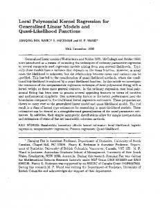
were less than one percent for all estimators, and are not presented. (The exceptions were percent relative design biases, in rare cases, of up to 12% for the model-based nonparametric procedures.) Table 1 shows the ratios of MSE's for the various estimators to the MSE for the local polynomial regression estimator with q = 1 (LPR1). Generally, both parametric and nonparametric regression estimators perform better than HT, regardless of whether the underlying model is correctly speci ed or not, but that eect decreases as the model variance increases. With a few exceptions, the model-based nonparametric estimators KERN and CDW have similar behavior in this study. With respect to design MSE, the model-assisted estimators LPR0 and LPR1 are sometimes much better and never much worse (MSE ratio 0:95) than the model-based estimators KERN and CDW. Similarly, LPR1 is sometimes much better and never much worse than LPR0 in this study, and so LPR1 emerges as the best among the nonparametric estimators considered here. Among the parametric estimators in this study, the higher-order parametric estimators (REG3 and PS) generally perform better than REG, except in the linear population. In most cases, LPR1 is competitive or better than the parametric estimators (MSE ratios 0:95). In several cases, the parametric estimators are somewhat better than LPR1 (MSE ratios 0.90{0.94). This is due to undersmoothing when the population is linear or quadratic and is due to oversmoothing in other cases. Finally, the PS estimator for the bump and cycle4 populations and the REG3 estimator for cycle1 are substantially better than the oversmoothed LPR1 estimator. In each of these cases, however, the LPR1 estimator at the smaller bandwidth is much better than the corresponding parametric estimator. Overall, then, the performance of the LPR1 estimator is consistently good, particularly at the smaller bandwidth. LPR1 loses a small amount of eciency relative to REG for a linear population, but dominates REG for other populations. It dominates the other nonparametric estimators considered here and it dominates the higher-order parametric estimators provided it is not oversmoothed. One common concern when using nonparametric regression techniques is how sensitive the results are to the choice of the smoothing parameter. This is especially important in the context of survey sampling, because the same set of regression weights (with a single choice for the bandwidth) are often used for a large number of dierent variables, as was done in the simulation experiment described above. A variable-speci c bandwidth selection procedure based on cross-validation is currently being investigated by the authors, and might be appropriate when the primary emphasis of a study is on achieving the best possible precision for a small number of variables. The investigation of such automated bandwidth selection procedures will be reported on elsewhere. As the bandwidth becomes large, the local linear regression estimator becomes equivalent

Local Survey Regression Estimators Population 0.1 linear 0.1 0.4 0.4 0.1 quadratic 0.1 0.4 0.4 0.1 bump 0.1 0.4 0.4 0.1 jump 0.1 0.4 0.4 0.1 cdf 0.1 0.4 0.4 0.1 exponential 0.1 0.4 0.4 0.1 cycle1 0.1 0.4 0.4 0.1 cycle4 0.1 0.4 0.4

h

0.10 0.25 0.10 0.25 0.10 0.25 0.10 0.25 0.10 0.25 0.10 0.25 0.10 0.25 0.10 0.25 0.10 0.25 0.10 0.25 0.10 0.25 0.10 0.25 0.10 0.25 0.10 0.25 0.10 0.25 0.10 0.25

19

HT REG REG3 PS LPR0 KERN CDW 33.35 0.90 0.94 1.43 0.98 0.98 0.95 35.41 0.95 1.00 1.52 1.45 1.68 0.98 2.97 0.90 0.94 1.05 0.96 0.95 0.95 3.16 0.95 1.00 1.12 1.00 1.02 0.98 2.96 3.02 0.94 1.15 0.99 1.02 1.08 3.08 3.14 0.98 1.20 1.29 2.16 2.70 1.01 1.02 0.94 1.03 0.96 0.95 0.96 1.07 1.08 1.00 1.10 1.00 1.07 1.11 25.06 4.90 4.00 2.08 1.13 1.50 1.47 8.57 1.67 1.37 0.71 1.13 1.32 1.14 3.43 1.35 1.30 1.15 0.98 1.01 1.01 2.94 1.16 1.11 0.98 1.01 1.07 1.03 7.12 5.24 2.08 1.51 1.00 1.08 1.07 4.88 3.59 1.42 1.03 1.13 1.53 1.46 1.47 1.30 1.05 1.07 0.96 0.95 0.95 1.51 1.33 1.07 1.09 1.00 1.05 1.04 6.37 3.00 1.64 1.20 1.00 1.02 1.02 5.00 2.35 1.29 0.94 1.09 1.44 1.58 1.58 1.05 0.97 1.05 0.98 0.97 0.97 1.64 1.09 1.01 1.08 1.00 1.04 1.08 5.21 2.90 1.07 1.36 1.10 1.19 1.19 4.88 2.72 1.00 1.27 1.64 2.44 2.45 1.14 1.02 0.96 1.05 0.97 0.96 0.96 1.20 1.07 1.00 1.10 1.03 1.10 1.10 46.58 18.68 1.36 2.73 1.24 1.46 1.25 16.15 6.48 0.47 0.94 1.66 2.55 2.34 3.91 2.08 0.99 1.15 0.97 0.97 0.96 3.67 1.95 0.93 1.08 1.09 1.26 1.23 3.85 3.79 3.56 1.83 1.21 1.97 2.02 0.98 0.96 0.91 0.46 1.09 1.00 1.09 2.27 2.26 2.17 1.35 1.07 1.42 1.45 0.97 0.97 0.93 0.58 1.07 1.01 1.08

Table 1: Ratio of MSE of Horvitz-Thompson (HT), linear regression (REG), cubic regression (REG3), poststrati cation (PS), local constant regression (LPR0), model-based kernel (KERN), and bias-calibrated nonparametric (CDW) estimators to local linear regression (LPR1) estimator, based on 1000 replications of simple random sampling from eight xed populations of size N = 1000. Sample size is n = 100. Nonparametric estimators are computed with bandwidth h and Epanechnikov kernel.


20

to the classical regression estimator, and the MSE's converge. Clearly, the bandwidth has an eect on the MSE of LPR1, but Table 1 suggests that large gains in eciency over other estimators can be gained for a variety of bandwidth choices. In particular, for either of the bandwidths considered here LPR1 essentially dominates HT for all populations and essentially dominates REG for all populations except linear, where it is competitive. This again shows that the local linear regression estimator is likely to be an improvement over Horvitz-Thompson and classical regression estimation when the relationship between the auxiliary variable and the variable of interest is non-linear. We have investigated the performance of the estimated variances from Corollary 1 relative to simulation variances. The ratios are generally close to one, though there is a fairly large amount of variability for sample size n = 100. The performance of the variance estimators for LPR1 is similar to the performance of variance estimators for REG in the cases we have examined. Further investigation of variance estimation for local polynomial regression estimators, including the use of the weighted residual technique (Sarndal, Swensson, and Wretman, 1989), will be reported elsewhere.

Appendix: Lemmas

Lemma 1 Assume A2 and A5. Then FN (x + hN ) ? FN (x ? hN ) ? f (x) ! 0 (15) 2hN as N ! 1, uniformly in x. Proof of Lemma 1: De ne DN = supx jFN (x) ? F (x)j. By A2 and the law of the iterated

logarithm (Ser ing, 1980, p. 62), DN satis es

2N 1=2DN = 1: (16) N !1 (2 log log N )1=2 Let > 0 be given. Then there exists > 0 such that jx?x0j < implies that jf (x)?f (x0)j < =2, by uniform continuity of f on [ax ; bx]. Using (16) and A5, choose N so large that N N implies that lim sup

2N 1=2DN < 1 + ; and (2 log log N )1=2 < : (17) hN < 2 ; (2 log 2(1 + ) log N )1=2 2N 1=2hN (Note that x0 2 (x ? hN ; x + hN ) implies that jx ? x0 j < 2hN < .) It follows that for any x, FN (x + hN ) ? F (x + hN ) + F (x ? hN ) ? FN (x ? hN ) 2hN 2h N + F (x + hN ) ? F (x ? hN ) ? f (x) 2hN F ( x + h D D N ) ? F (x ? hN ) N N ? f (x) 2h + 2h + 2hN N N


21

2N 1=2DN (2 log log N )1=2 + jf (x ) ? f (x)j N (2 log log N )1=2 2N 1=2hN (1 + ) 2(1 + ) + 2 = ; =

(18)

where the equality in (18) holds for some xN 2 (x ? hN ; x + hN ) by the mean value theorem. The uniform convergence in Lemma 1 has a number of useful consequences.

Lemma 2 Under A1{A6, (i) for k 0,

0 X @ 1 X Ifxi?hN xj xi lim sup N1 2Nh N !1

N j 2UN

i2UN

1k hN g A < 1

+

(ii) there exists N , independent of x, such that N N implies X Ifjx?xk jhN g q + 1 k2UN

(iii) the N ? tig are uniformly bounded in i and the N ? tîg are uniformly bounded in i and s (iv) the mi are uniformly bounded in i and the m^ i are uniformly bounded in i and s (v) the rst, second, third, and fourth order mixed partials of m^ i with respect to N ? tig and , evaluated at ^ti = ti , = 0, are uniformly bounded in i (vi) the RiN are uniformly bounded in i and s 1

1

1

2

Proof of Lemma 2: (i). By Lemma 1,

1k

0

X@ 1 X Ifxi?hN xj xi+hN g A lim sup N1 2 Nh N N !1 j 2UN i2UN

)k X ( FN (xi + hN ) ? FN (xi ? hN ) 1 ? f (xi) + f (xi) lim sup N 2hN N !1 i2UN X lim sup 1 f + f (x )gk N !1

< 1:

N i2UN

i


22

(ii). If not, then we could set = minx f (x)=2 > 0 by compactness of the support and continuity of f , and choose N so large that N N satis es (17) and implies (q + P 1)=(2NhN ) < . For some x and some N N , k2UN Ifjx?xk jhN g < q + 1, so that

f (x) ?

P

k2UN Ifjx?xk jhN g

2NhN

+1 > f (x) ? 2qNh

N

minx f (x) = ; > min f ( x ) ? x 2 contradicting the uniform convergence in (15). (iii). Under the given assumptions,

X xk ? xi I 1 k p p1 y 2 K ( x ? x ) lim sup jN ? tîg j = lim sup k i k k hN N !1 k2UN NhN N !1 X c lim sup Nh Ifxi?hN xk xi hN g; 1

N !1 k2UN

N

+

which does not depend on s, and is bounded independently of i by Lemma 1. Since < 1, the same uniform bound works for N ?1tig . (iv), (v), (vi). The mi are continuous functions of the uniformly bounded tig , with denominators uniformly bounded away from zero by (ii) above. Similarly, the m ^ i and ^ their derivatives are continuous functions of the uniformly bounded tig , with denominators uniformly bounded away from zero by the adjustment in (8). Combining these results and using the de nition in (10), the R2iN are uniformly bounded in i and s.

Lemma 3 Assume A1{A7. For the Taylor linearization remainders of the sample local polynomial residuals in equation (10),

nN X E hR2 i = O 1 : N i2UN p iN nN h2N

Proof of Lemma 3: Note that

n2N h2N X E jN ?1 (t^ ? t )j4 ig ig N i2UN p 2 2 X cn h N N Ifxi?hN xj ;xk;x`;xm xi +hN g Ep [(Ij ? j )(Ik ? k )(I` ? ` )(Im ? m)] N 5 h4 N i;j;k;`;m2UN

c hN nN j;k;`;m max2D Ep [(Ij ? j )(Ik ? k )(I` ? ` )(Im ? m )] 4;N 0 1 X X I fxi ?hN xj xi hN g A @ 1 1

2

2

(

)

4

N i2UN j2UN

NhN

+


23

h i 2 N hN 2 nN (j;k;`max ( I ? ) ( I ? )( I ? ) E +c2 nNh j j k k ` ` p )2D3;N N 1 0 X @ X Ifxi?hN xj xi +hN g A3 1 N NhN i2UN j 2UN 0

1

2 2 X @ X Ifxi?hN xj xi +hN g A +c3 nN2hN2 1 N hN N i2UN j2UN NhN 0 1 2 2 X X I 1 n h fxi ?hN xj xi +hN g A @ ; +c4 N3 N3 N hN N i2UN j2UN NhN 2

which remains bounded by A5, A7, and Lemma 2(i). The assumptions ofPTheorem 5.4.3 of Fuller (1996) with = 1, s = 4, aN = O((nN hN )?2 ), and expectation N ?1 i2UN Ep [] are then met for the sequence fR2iN g. Since this function and its rst three derivatives with respect to the elements of (N ?1ti ; ) evaluate to zero, we conclude that nN X E hR2 i = O 1 ; which goes to zero by A5.

p

N i2UN

iN

nN h2N

Lemma 4 Assume A1{A7. Then

1 X E (m 2 lim p ^ i ? mi ) = 0: N !1 N i2UN

Proof of Lemma 4: By (10), 1 X E (m 2 p ^ i ? mi ) =

N i2UN

1 X X z z kl ? k l ik i` N3 k l i2UN k;`2UN

Ik X 2 + 2 zik Ep 1 ? RiN N

+ N1

i;k2UN

X

h

i

k

Ep R2iN + o N 2 ; i2UN

(19)

where the remainder term o(N ?2 ) comes from the expansion (10) and does not depend on the sample. By Lemma 1 and Lemma 2(v), 1 X z2 c X I !0

N 3 i;k2UN

ik

N 3h2N i;k2UN fxi?hN xk xi +hN g


24

as N ! 1. Thus, following the argument of Theorem 1 in Robinson and Sarndal (1983), the rst term of (19) is 1 X X z z k` ? k `

N 3 i2UN k;`2UN

ik i`

k ` X X 2 1 ? k 1 X X = N13 zik zi` k`?k ` zik + N 3 k k ` i2UN k2UN i2UN k6=` X 2 N maxi;j2UN :i6=j jij ? ij j X 2 zik + zik ; N1 3 2 N 3 i;k2UN i;k2UN

which converges to zero using A6. The last term of (19) converges to zero by Lemma 3, and the second term converges to zero by an application of the Cauchy-Schwarz inequality.

Lemma 5 Assume A1{A7. Then 2 nN 4 X

!3

Ij 5 = 0: I i E 1 ? ( m ^ ? m )( m ^ ? m ) 1 ? lim p i i j j 2 N !1 N i j i;j 2UN

Proof of Lemma 5: By (10),

2

!3

nN E 4 X (m^ ? m )(m^ ? m ) 1 ? Ii 1 ? Ij 5 N 2 p i;j2UN i i j j i j " ! I # X I I I n i k j N zik zj` Ep 1 ? 1 ? 1 ? 1 ? ` = N4 i j k ` i;j;k;`2UN # ! " X zik Ep RjN 1 ? Ii 1 ? Ij 1 ? Ik + 2NnN3 i j k i;j;k2UN " !# nN X E R R 1 ? Ii 1 ? Ij + o(1) +N p iN j N 2 i j i;j 2UN = b1N + b2N + b3N + o(1):

The remainder term o(1) comes from the O(N ?2) term in (10), using the Cauchy-Schwarz inequality for its two cross-products. In b1N , we consider separately the cases of one, two, three, and four distinct elements in (i; j; k; `). Straightforward bounding arguments like those in Lemma 3 show that each such case converges to zero. We omit the details. The term b3N converges to zero by Lemma 3 and A6. The cross-product term b2N goes to zero by an application of the Cauchy-Schwarz inequality, and the result is proved.


Lemma 6 Under A1{A5, lim N ?1 N !1

X i2UN

25

E (mi ? m(xi ))2 = 0:

Proof of Lemma 6: This follows directly from standard local polynomial regression theory (e.g. Wand and Jones, 1995, p. 125).

Lemma 7 Assume A1{A7. Then,

nN lim N !1 N

X h i2UN

i

E R2iN = 0:

Proof of Lemma 7: The proof is identical to that of Lemma 3, after replacing the P ? 1 expectation operator with N i2UN E [], because the uniformity results of Lemma 1 and Lemma 2 hold not only for all i 2 UN and s, but also across realizations from .

Lemma 8 Assume A1{A7 hold. Then, 2 !3 X (m^ i ? mi )(m ^ j ? mj ) 1 ? Ii 1 ? Ij 5 = 0: lim nN E 4 N !1 N i j i;j 2UN 2

Proof of Lemma 8: The result follows from the assumptions and Lemma 7, using bounding arguments exactly as in Lemma 5.

Acknowledgements We are grateful to four anonymous referees for numerous constructive suggestions. This work was supported in part by cooperative agreement 68{3A75{43 between the USDA Natural Resources Conservation Service and Iowa State University. Computing for the research reported in this paper was done with equipment purchased with funds provided by an NSF SCREMS grant award DMS 9707740.

References Brewer, K.R.W. (1963). Ratio estimation in nite populations: some results deductible from the assumption of an underlying stochastic process. Australian Journal of Statistics 5, 93{105.


26

Cassel, C.-M., Sarndal, C.-E., and Wretman, J.H. (1977). Foundations of Inference in Survey Sampling. Wiley, New York. Chambers, R.L. (1996). Robust case-weighting for multipurpose establishment surveys. Journal of Ocial Statistics 12, 3{32. Chambers, R.L., Dorfman, A.H., and Wehrly, T.E. (1993). Bias robust estimation in nite populations using nonparametric calibration. Journal of the American Statistical Association 88, 268{277. Chen, J. and Qin, J. (1993). Empirical likelihood estimation for nite populations and the eective usage of auxiliary information. Biometrika 80, 107{116. Cleveland, W.S. (1979). Robust locally weighted regression and smoothing scatterplots. Journal of the American Statistical Association 74, 829{836. Cleveland, W.S., and Devlin, S. (1988). Locally weighted regression: an approach to regression analysis by local tting. Journal of the American Statistical Association 83, 596{610. Cochran, W.G. (1977). Sampling Techniques, 3rd ed. Wiley, New York. Deville, J.-C. and Sarndal, C.-E. (1992). Calibration estimators in survey sampling. Journal of the American Statistical Association 87, 376{382. Dorfman, A.H. (1992). Nonparametric regression for estimating totals in nite populations. Proceedings of the Section on Survey Research Methods, American Statistical Association, 622{625. Dorfman, A.H. and Hall, P. (1993). Estimators of the nite population distribution function using nonparametric regression. Annals of Statistics 21, 1452{1475. Fan, J. (1992). Design-adaptive nonparametric regression. Journal of the American Statistical Association 87, 998{1004. Fan, J. (1993). Local linear regression smoothers and their minimax eciencies. Annals of Statistics 21, 196{216. Fan, J. and Gijbels, I. (1996). Local Polynomial Modeling and its Applications, Chapman and Hall, London. Fuller, W.A. (1996). Introduction to Statistical Time Series, second edition. Wiley, New York. Godambe, V.P. and Joshi, V.M. (1965). Admissibility and Bayes estimation in sampling nite populations, 1. Annals of Mathematical Statistics 36, 1707{1722. Hall, P. and Turlach, B.A. (1997). Interpolation methods for adapting to sparse design in nonparametric regression. Journal of the American Statistical Association 92, 466{472. Hastie, T.J. and R.J. Tibshirani. (1990). Generalized Additive Models, Chapman and Hall, London. Horvitz, D.G. and D.J. Thompson. (1952). A generalization of sampling without replacement from a nite universe. Journal of the American Statistical Association 47, 663{685. Isaki, C.T. and Fuller, W.A. (1982). Survey design under the regression superpopulation model. Journal of the American Statistical Association 77, 89{96.


27

Kuo, L. (1988). Classical and prediction approaches to estimating distribution functions from survey data. Proceedings of the Section on Survey Research Methods, American Statistical Association, 280{285. Opsomer, J.-D., and Ruppert, D. (1997). Fitting a bivariate additive model by local polynomial regression. Annals of Statistics 25, 186{211. Pollard, D. (1984). Convergence of Stochastic Processes. Springer, New York. Robinson, P.M. and Sarndal, C.-E. (1983). Asymptotic properties of the generalized regression estimation in probability sampling. Sankhya: The Indian Journal of Statistics, Series B 45, 240{248. Royall, R.M. (1970). On nite population sampling under certain linear regression models. Biometrika 57, 377{387. Ruppert, D., and Wand, M.P. (1994). Multivariate locally weighted least squares regression. Annals of Statistics 22, 1346{1370. Sarndal, C.-E., Swensson, B., and Wretman, J. (1989). The weighted residual technique for estimating the variance of the general regression estimator of the nite population total. Biometrika 76, 527{537. Sarndal, C.-E., Swensson, B., and Wretman, J. (1992). Model Assisted Survey Sampling, Springer, New York. Sarndal, C.-E. (1980). On -inverse weighting versus best linear unbiased weighting in probability sampling. Biometrika 67, 639{650. Sen, P.K. (1988). Asymptotics in nite population sampling. In: P.R. Krishnaiah and C.R. Rao (eds) Handbook of Statistics, Vol. 6. North-Holland, Amsterdam, 291{331. Ser ing, R.J. (1980). Approximation Theorems of Mathematical Statistics, Wiley, New York. Tam, S.M. (1988). Some results on robust estimation in nite population sampling. Journal of the American Statistical Association 83, 242{248. Thompson, M.E. (1997). Theory of Sample Surveys, Chapman and Hall, London. Wand, M.P. and Jones, M.C. (1995). Kernel Smoothing, Chapman and Hall, London. Wright, R.L. (1983). Finite population sampling with multivariate auxiliary information. Journal of the American Statistical Association 78, 879{884.