Localization in Wireless Sensor Networks: A Probabilistic ... - CiteSeerX

Localization in Wireless Sensor Networks: A Probabilistic Approach Vaidyanathan Ramadurai, Mihail L. Sichitiu Department of Electrical and Computer Engineering North Carolina State University Raleigh, NC 27695 email: {vramadu,mlsichit}@ncsu.edu

Abstract— In this paper we consider a probabilistic approach to the problem of localization in wireless sensor networks and propose a distributed algorithm that helps unknown nodes to determine confident position estimates. The proposed algorithm is RF based, robust to range measurement inaccuracies and can be tailored to varying environmental conditions. The proposed position estimation algorithm considers the errors and inaccuracies usually found in RF signal strength measurements. We also evaluate and validate the algorithm with an experimental testbed. The test bed results indicate that the actual position of nodes are well bounded by the position estimates obtained despite ranging inaccuracies.

Keywords: Localization, wireless sensor network, RSSI, probabilistic, distributed, range inaccuracy, position estimates. I. I NTRODUCTION A wireless sensor network is a distributed collection of nodes which are resource constrained and capable of operating with minimal user attendance. Some of the potential applications of wireless sensors include environmental monitoring, military surveillance, search-and-rescue operations, tracking patients and doctors in a hospital and other commercial applications. Wireless sensor nodes operate in a cooperative and distributed manner. Such nodes are usually embedded in the physical environment and report sensed data to a central base station; however, for a sensor network to achieve its purpose, it is essential to know where the information is sensed. We define the problem of localization as estimating the position or spatial coordinates of wireless sensor nodes. Localization is an inevitable challenge when dealing with wireless sensor nodes, and a problem which has been studied for many years. Nodes can be equipped with a Global Positioning System (GPS) [1], but this is a costly solution in terms of volume, money and power consumption. While much research has focused on developing different algorithms for localization, less attention has been paid to the problem of range measurement inaccuracy. In this paper, we discuss a robust and distributed RSSI-based position estimation algorithm for wireless sensor network in the presence of range measurement inaccuracy. Our approach This work was supported by NC State University Faculty Research and Development Grant.

is probabilistic and can be easily geared to various environmental conditions by recalibrating the system or sacrificing accuracy. II. R ELATED W ORK Recently, there has been an increasing interest in indoor localization systems. The RF based RADAR [2] system can track users within a building, while the Cricket [3] location support system uses ultrasound instead for indoor localization. Directional approaches considering steerable directional antennas have been explored in [4], [5]. An interesting idea is explored in [6] where the problem of localization is considered in the absence of beacons, while a method for estimating unknown node positions in a sensor network based on connectivity-induced constraints is described in [7]. In [8], experimental evaluation of localization systems with beacon density is considered an important parameter in determining localization quality. Several other localization algorithms have been proposed and implemented for outdoor localization [9]–[13]. None of those systems used a probabilistic approach to find the positions of the nodes. Instead they rely on accurate range measurements. Accurate measurements are possible using an acoustic ranging technique [10], but almost impossible with RF signal strength measurements. The only other localization techniques using a probabilistic approach were conducted for indoor systems [14]–[16] where the multipath fading make predicting the range as a function of the signal strength practically impossible. To overcome this problem, the authors had to calibrate the system in every spot of an entire building, which is clearly undesirable for a wireless sensor network environment, which may be hostile or inaccessible. III. P ROPOSED A PPROACH In this section, we present a probabilistic position estimation algorithm that consider range measurement inaccuracies. Nodes in a sensor network can belong to two different classes, namely beacons and unknowns. We assume that the beacons have known positions (either by being placed at known positions or by using GPS), while the unknown nodes estimate

0.25

0.2

Probability distribution function

their position with the help of beacons. The first step in RF-based localization is range measurement, i.e estimating the distance between two nodes, given the signal strength received by one node from the other. RF-based signal strength measurements are usually prone to inaccuracies and errors and, hence, calibration of such measurements is inevitable before using them for localization. For this algorithm to work, extensive preliminary field measurements and calibrations were carried out as discussed in the following subsections.

0.15

0.1

0.05

0

Fig. 1.

0

5

10

15

20

25 Distance

30

35

40

45

50

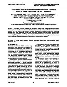
Distribution of distances for a received signal strength of 70.

A. Measurements and Data Collection

B. Processing of Data Collected We merged all of the data collected and calculated the probability distribution of each signal strength as a function of distance. Interestingly, the probability distribution followed a normal distribution for most of the signal strengths. We also note that there might be better distributions that could fit the data collected; however, the focus of our research is primarily on implementing and testing the functionality of the algorithm rather than developing optimum distributions to fit the data. The position estimation algorithm that we discuss later in this paper is independent of the type of distribution as long as there exists a feasible way to represent it in a compact fashion. Fig. 1 shows a graph with a normal fit for data collected with a received signal strength of 70. The mean and standard deviation for each signal strength was noted and tabulated as a function of distance. A graphical view of the table is shown in Fig. 2 for signal strengths ranging from 66 to 90. The proposed algorithm, which is described in the next section, uses this table for ranging; i.e., any node receiving a beacon packet will estimate itself to be located on a surface that has a probability distribution dictated by the mean and standard deviation corresponding to the signal strength received. The measurements we collected were for an outdoor environment with very little interference. It is pretty clear that in conditions where RF measurements are severely hampered by interference and other environmental factors, we can increase the probability distribution factor (in this case, the standard

0.45 0.4 0.35 0.3 0.25 pdf

To evaluate the accuracy of RSSI measurements, we used two HP Compaq H3870 iPAQs equipped with Lucent Orinoco cards to measure the signal strength as a function of distance. One of the iPAQs was configured to send beacon packets continuously while the other was measuring the signal strength of each received packet. The two iPAQs were placed in an outdoor field and remotely controlled from a laptop. We measured the signal strength and noise in intervals of 2.5m up to 50m. For each distance, we measured the data at 16 different positions (the sender was rotated by 90 degrees, for each position of the sender, the receiver was rotated by 90 degrees). We took 200 measurements at each position for a total of 3200 measurements at every distance. We noted a significant change in signal strength as a function of distance, while the noise remained almost the same; so, we considered only the signal strength information in our analysis.

0.2 0.15 0.1 0.05 0 80 90

60 85

40

80 75

20 70 Distance

Fig. 2.

0

65

Signal Strength

Probability distribution of signal strength with distance.

deviation) to account for deviations from the actual or mean position estimate. Sensors can dynamically adapt and tune to such changing environments by choosing the right parameters to localize themselves. However, we focus our interest only on the outdoor environment localization problem in this paper. Indoors, it is likely that the proposed method will work with very poor accuracy. C. Algorithm Consider Fig. 3(a) which shows two beacons (1 and 2) assisting an unknown node (3). With a Gaussian distribution as indicated by our measurements, the unknown node will estimate its final position as shown in Fig. 3(b). A threedimensional view of the same position estimate is shown in Fig. 3(c). The nodes are more likely to be towards the mean, and accordingly, their probability distributions are higher towards the mean. Each point on every surface will have a real positive value representing the probability distribution function associated with that surface. A higher value at position (x, y) represents a higher probability that the node is at the coordinates (x, y). Every unknown node in the network will execute a distributed algorithm as follows: The unknown node initializes its position estimate to the entire space. The node then waits to receive beacon packets from its neighboring nodes, and upon receiving a beacon packet, updates its position estimate by computing the constraint and intersects it with the current estimate to obtain the new estimate. If the position estimate improves, it will wait for a specific period of time and will broadcast its new estimate to all of its neighbors. Every node receives a beacon packet either directly from a beacon or from another unknown node. Each such packet

3

3

1

2

1

(a)

2

(b)

(c)

Fig. 3. (a) Two beacons (1 and 2) assisting an unknown node (3). (b) The resulting position estimate. (c) The same constraints and position estimate as in (a) and (b) represented as 3D surfaces.

Node Type

Node ID

Fig. 4.

Total Length

Position estimate

Length

Beacon ID

Peer ID

X coordinates

Y coordinates

mean1

stdev1

mean2

stdev2

.....

Length

Beacon ID

Peer ID

X coordinates

Y coordinates

mean1

stdev1

mean2

stdev2

.....

Packet format of a beacon message. Fig. 6.

contains a position estimate field of the node originating the packet as shown in Fig. 4. If the message comes directly from a beacon, the position estimate is a point (ideal case) or a very small area (corresponding to uncertainty in GPS measurements). In this case, the constraint is simple. If the unknown node estimates a mean µ and standard deviation σ from the signal strength of the beacon message, the constraint is a Gaussian normal distributed surface of mean µ and standard deviation σ. This is equivalent to a Gaussian function rotated 360 degrees around the coordinates of the beacon. Fig. 5 shows the constraint imposed by a beacon on an unknown node after transmitting a beacon message.

Fig. 5.

Constraint imposed by a beacon on an unknown node.

On the other hand, if the message comes from another unknown node, the constraint is not necessarily Gaussian. We will explore how the constraint is computed by an unknown node in such a situation in Section III-E. D. Algorithm Design and Implementation Issues The beacon packet format described in the previous section is a generic format. The position estimate sent by a beacon is not the same as the one sent by an unknown node as part of the beacon message. In the case of beacons, the position estimate is a point (x, y), while it is an estimate in the case

Format of the position estimate as stored by an unknown node.

of an unknown. We used the following method to store the position estimate at each unknown node. Upon receiving a beacon packet, every unknown node records the beacon ID, the peer that originated the message and the estimated mean and standard deviation for that peer. In this way, a cascade of distribution is stored and transmitted by every unknown node in the network. Thus the position estimate field will, look as shown in Fig. 6. Only two rows are shown; the total size depends on the number of beacons in the network. We note that there might be multiple entries (rows) for a single beacon, when a node receives beacon messages from different neighbors for a particular beacon ID. Finally, the length of each cascade depends on the size of the network diameter. If we assume the maximum distance between any two unknown nodes as k hops, then the size will not exceed (4k + 8) bytes, assuming that each field takes 2 bytes. We observe that there are a number of other ways to store position estimates and transmit them to other unknown nodes in the network. One method is the grid approach, where the network space is divided into a uniform grid, and the probability is estimated at each square in the grid. This method has obvious drawbacks because of storage and memory requirements. The finer the grid, the greater the memory required to store the estimates. There is a clear tradeoff between the precision of the position estimate and the storage requirement. Wireless sensor nodes usually have limited memory resources, and the grid representation would consume most of those resources. Transmitting position estimates as a cascade of distributions and having the unknown nodes compute the estimates locally guarantees lesser memory requirements and allows the nodes to obtain more precise estimates. When a beacon sends a beacon packet, all of its neighbors may update their position estimates; and, in return, each sends a beacon packet, which will reach the neighbor’s neighbors and will keep multiplying. In reality, fewer numbers of beacon messages propagate in the network and, hence, maintain the locality of the algorithm.

7 for (every unknown node) open the log file; initialize the position estimate P to the entire space;

8

2

for (every row in the file) initialize constraint C to NULL; set pointer to mean1;

1 3 5

while(!endof(row)) read mean, stdev; compute new constraint N; C = C + N; increment pointer to point to the next mean; end while;

6

4 Fig. 7. The information from beacon node 1 is aggregated at node 5 and only one beacon message is sent to nodes 6 and 8.

P = P

C;

end for; end for;

An important observation is that the only nodes which actually provide information in the system are the beacons. All of the other nodes simply relay these primary sources of information. Consider the situation depicted in Fig. 7. The information from beacon node 1 reaches nodes 2, 3 and 4. In turn, each of the nodes 2, 3 and 4 will broadcast its newlycomputed position estimate. Node 5 will receive each of the broadcasts, and it can aggregate the information from all three broadcasts before sending out its own update. Then, node 8 and 6 will only receive one broadcast from node 5. In our implementation, a main process spawns four threads, namely recv beacon, send beacon, recv rssi and send rssi. The recv beacon thread waits for beacon packets and, upon receiving one, updates its estimate and puts it into the queue to be broadcast. When the aggregation timer expires, the send beacon thread dequeues the packet and broadcasts it to its neighbors. Ranging based on signal strength measurements can be very irregular and uncertain due to multipath fading and interference, despite extensive field measurements. A single bad beacon message received (in this case a higher or lower signal strength than the one expected) can result in incorrectness and deviation from the original position estimate. To increase the robustness of the algorithm, we take multiple signal strength measurements between pairs of nodes. The send rssi thread sends an RSSI packet every second. The recv rssi thread waits for an RSSI packet from its neighbors and estimates the signal strength of this packet. Then it calculates the mean and standard deviation as indicated before from the signal strength table. When a subsequent packet is received with a particular signal strength, it shifts the mean and standard deviation based on a weighted formula. If (µ1 ,σ1 ) and (µ2 ,σ2 ) are the two consecutive measurements, then the new shifted measurement (µshif t ,σshif t ) is computed as: µshif t =

µ1 σ22 + µ2 σ12 σ12 + σ22 σ1 σ2

σshif t = p

σ12 + σ12

(1)

(2)

Fig. 8. The algorithm executed by each node to calculate the estimates of unknown nodes.

The nodes were run until they estimated, with high confidence, a position with the smallest area. One method of deciding when such a position estimate is obtained is by computing the ”spikiness” of localization. A practical way to do this is to find the area that contains the node with 99% confidence. If this area is considerably smaller than the previous estimate, it triggers an update. But, in this experiment, we let the nodes run for enough time to ensure that they get all the beacon messages needed to localize themselves. We also logged the position estimate of every unknown node after each update. The log format was the same as the format of the position estimate as shown in Fig. 6. The logs collected were then transferred to a central computing unit (CU) that processed them to calculate the position estimate of each node in stages. In the real deployment, every unknown node can run the CU program to estimate its own position, as each node has all the information it needs to localize itself. E. Computation of Final Estimates Initially, we assume that every node in the network is present in the entire space with equal probability. We also assume that the network is fully connected, although our algorithm will also work in partitioned networks. The CU will execute the pseudocode shown in Fig. 8. The CU processes each row in the log of every unknown node to obtain the constraints and updates the current estimate by intersecting it with the old position estimate. We will shortly explain what the addition and intersection symbols in the algorithm actually mean. As discussed before, if the beacon message is directly from a beacon, the constraint C(x, y) imposed on the unknown node is given by a Gaussian normal distributed surface around the coordinates of the beacon. Thus, the unknown node updates its position estimate by intersecting the old position estimate P (x, y) with the constraint C(x, y).

(a)

(b)

(c)

(d)

Fig. 9. (a) Constraint after the beacon message travels one hop. (b) Constraint after the beacon message travels two hops. (c) Old position estimate of an unknown node. (d) New estimate obtained by intersecting the constraint with the old estimate.

If the beacon message is from an unknown node, the CU has to process the cascade of distributions before intersecting with the old position estimate. The new constraint is calculated by adding the individual constraints. The sum of these constraints is similar to the convolution of all the individual distributions. Assume that we have a beacon at coordinates (xb , yb ) and two unknown nodes 1 and 2. Assume that, corresponding to the signal strength that node 1 receives from the beacon we have the pdf function f1 (d) (e.g., a Gaussian with parameters µ1 and σ1 ); and similarly, corresponding to the signal strength that node 2 receives from node 1 we have the pdf function f2 (d). Then, the position estimate of node 1 is given by: E1 (x, y) = f1 (d(x, y), (xb , yb ))

∀(x, y),

1 8

7 60

2

3 4

10

50

13 12

40 11

14

30

60

5 50 20

40 30

Y meters

10

20 10 0

Fig. 10.

X meters 0

Experiment Configuration.

(3)

where d(A, B) is the Euclidean distance between points A and B. The position of node 2 is given by (4). Fig. 9 (b) shows the convolution of two constraints. Fig. 9 (a) shows how the constraint looks after a beacon message has traveled one hop from a beacon centered at (xb = 36m, yb = 37m) with received estimated Gaussian parameters of µ = 17.65, σ = 2.147 at unknown node 1, while Fig. 9 (b) shows the resultant constraint after it traverses another hop with received estimated Gaussian parameters of µ = 18.265, σ = 2.889 at node 2. If constraint in Fig. 9(b) is the first constraint obtained by node 2, then the new position estimate is the same as the constraint (since the constraint is intersected with the initial uniform distribution). Otherwise, the constraint is intersected with the old estimate of node 2 as shown in Fig. 9 (c) to produce a new estimate as presented in Fig. 9 (d). Every row in the log file is a constraint which is intersected with the old position estimate to calculate the current estimate. P (x, y) × C(x, y) P (x, y) = R ∞ R ∞ P (x, y) × C(x, y)dxdy −∞ −∞

6

(5)

IV. E XPERIMENTAL E VALUATION Our experimental test bed consists of nodes scattered randomly in a field of size (60m × 60m). We used 5 beacons and 8 unknown nodes to test the algorithm. We chose HP Compaq H3870 iPAQs running Familiar distribution of Linux [17], equipped with a 11 Mbps Lucent Orinoco card as our test bed nodes. We restricted the range of each node to 20m

by ignoring messages with the signal strength below a certain threshold. All the nodes were controlled from a central unit to which the logs were transferred after the nodes localized themselves. The set up of our experimental test bed is shown in Fig. 10. The red circles indicate beacons while the black circles indicate unknown nodes. We observe that the network is sparse with many unknown nodes having close proximity to only one or two beacons. The beacons were configured to send beacon packets continuously every 1s. The position information of each beacon was hard coded with the help of a GPS. On average the GPS had an accuracy of 5m, which was considered in the end after the nodes estimated their positions. Fig. 11 shows the results of our experiment. The top view shows the comparison of position estimates obtained with the actual estimates. The circular ring indicates the GPS accuracy associated with the actual position of an unknown node. The side view provides a better indication of sharpness in the position estimate of unknown nodes. Some nodes like 7, 12, 10 and 8 establish a very precise estimate; while nodes like 13 (of all nodes) have inaccurate position estimates (expected when using inaccurate measurements). The error of the final position estimates is shown in Fig. 12. Considering the 7-8m error of the GPS receiver, the results are surprisingly good. A graph showing the improvement in the position estimate of each unknown node after receiving a beacon packet is shown in Fig. 13. The graph shows the area enclosing the node

R E2 (x, y)

=

R

R x2

=

R

R

y2

R x2

x2

R

x1

x2

R R

y2

R x1

R

x1

R

x1

E1 (x1 , y1 )f2 (d((x, y), (x1 , y1 )))dx1 dy1

x2

f1 (d(x1 , y1 ), (xb , yb ))f2 (d((x, y), (x1 , y1 )))dx1 dy1

f (d(x1 , y1 ), (xb , yb ))f2 (d((x2 , y2 ), (x1 , y1 )))dx1 dy1 dx2 dy2 x2 1

(a) Fig. 11.

(4)

E1 (x1 , y1 )f2 (d((x2 , y2 ), (x1 , y1 )))dx1 dy1 dx2 dy2

(b)

(c)

(a) Position estimate of Nodes 11, 7 and 13. (b) Position estimate of Nodes 10, 12 and 6. (c) Position estimate of Nodes 14 and 8.

4

20

10

18

Area of the estimate (m ) − 95% confidence

16

12

2

Position error [m]

14

10

8

6

3

10

4

2

0

Fig. 12.

0

2

4

6

8

10 Node ID

12

14

16

18

20

The localization error for each of the unknown nodes.

0

1

2

3 4 5 No. of beacon messages received

6

7

8

Fig. 13. Improvement in the position estimate of nodes with the number of beacon packets received.

V. C ONCLUSION with 95% confidence. From the position estimates shown in Fig. 11 and the graph in Fig. 13, we infer that nodes having smaller final estimates in terms of area are not necessarily the ones having precise estimates. For example, from the graph, node 6 has the best final position estimate in terms of area, but lies within the low probability density area; yet, the position estimates obtained bound the actual positions of all nodes exceedingly well.

In this paper, we have described a novel, robust and distributed algorithm for localizing nodes in sensor networks. The approach is RSSI based and takes range measurement inaccuracies into account, which, according to our knowledge, have not yet been pursued in literature. Our extensive outdoor field measurements and calibration indicate that a received signal strength is inaccurate and the proposed approach uses this information directly for ranging. Also, the algorithm

is independent of the type of distribution as long as there exists a feasible and practical method to store and compute the distributions. The proposed algorithm can be tailored to varying environmental conditions by changing the probability distribution parameter that accounts for deviation from the mean position estimate. Our experimental testbed analysis has also shown positive results with the nodes being well bounded by the estimates obtained. R EFERENCES [1] B. Hofmann-Wellenhof, H. Lichtenegger, and J. Collins, Global Positioning System: Theory and Practice, Springer-Verlag, 4th edition, 1997. [2] P. Bahl and V. Padmanabhan, “RADAR: An in-building RF-based user location and tracking system,” in Proc. of Infocom’2000, Tel Aviv, Israel, Mar. 2000, vol. 2, pp. 775–584. [3] N. Priyantha, A. Chakraborthy, and H. Balakrishnan, “The cricket location-support system,” in Proc. of International Conference on Mobile Computing and Networking, Boston,MA, Aug. 2000, pp. 32– 43. [4] C. Savarese, J. M. Rabaey, and J. Beutel, “Locationing in distributed ad-hoc wireless sensor networks,” in Proc. of ICASSP’01, 2001, vol. 4, pp. 2037–2040. [5] A. Nasipuri and K. Li, “A directionality based location discovery scheme for wireless sensor networks,” in First ACM International Workshop on Wireless Sensor Networks and Applications, Atlanta, GA, Sept. 2002. [6] S. Capkun, Maher Hamdi, and J. P. Hubaux, “GPS-free positioning in mobile ad-hoc networks,” Cluster Computing, vol. 5, no. 2, April 2002. [7] L. Doherty, K. S. J. Pister, and L. El Ghaoui, “Convex position estimation in wireless sensor networks,” in Proc. IEEE Infocom 2001, Anchorage AK, Apr. 2001, vol. 3, pp. 1655–1663. [8] D. Estrin N. Bulusu, J. Heidemann and Tommy Tran, “Self-configuring localization systems: Design and experimental evaluation,” in ACM Transactions on Embedded Computing Systems (ACM TECS), 2003. [9] N. Bulusu, J. Heidemann, and D. Estrin, “GPS-less low cost outdoor localization for very small devices,” IEEE Personal Communications Magazine, vol. 7, pp. 28–34, Oct. 2000. [10] L. Girod and D. Estrin, “Robust range estimation using acoustic and multimodal sensing,” in Proceedings of the IEEE/RSJ International Conference on Intelligent Robots and Systems (IROS 2001), Maui, Hawaii, Oct. 2001. [11] A. Savvides, C. C. Han, and M. B. Srivastava, “Dynamic fine-grained localization in ad-hoc networks of sensors,” in Proc. of Mobicom’2001, Rome, Italy, July 2001, pp. 166–179. [12] K. Whitehouse and D Culler, “Calibration as parameter estimation in sensor networks,” in First ACM International Workshop on Wireless Sensor Networks and Applications, Atlanta, GA, Sept. 2002. [13] Andreas Savvides, Heemin Park, and Mani Srivastava, “The bits and flops of the n-hop multilateration primitive for node localization problems,” in First ACM International Workshop on Wireless Sensor Networks and Applications, Atlanta, GA, Sept. 2002. [14] P. Bahl and V. N. Padmanabhan, “Enhancements to the radar user location and tracking system,” in Microsoft Research Technical Report MSR-TR-2000-12, 2000. [15] Andrew M. Ladd, Kostas E. Bekris, Guillaume Marceau, Algis Rudys, Lydia E. Kavraki, and Dan Wallach, “Robotics-based location sensing using wireless ethernet,” in Proc. of Eighth ACM International Conference on Mobile Computing and Networking (MOBICOM 2002), Atlanta, Georgia, Sept. 2002. [16] M. Hel´en, J. Latvala, H. Ikonen, and J. Niittylahti, “Using calibration in RSSI-based location tracking system,” in Proc. of the 5th World Multiconference on Circuits, Systems, Communications & Computers (CSCC20001), 2001. [17] “The familiar project, http://familiar.handhelds.org.,” .