Maximum Mipmaps for Fast, Accurate, and Scalable ... - Art Tevs

Maximum Mipmaps for Fast, Accurate, and Scalable Dynamic Height Field Rendering Art Tevs, Ivo Ihrke and Hans-Peter Seidel Max-Planck-Institut für Informatik

Figure 1: Left: Scene rendered with around 40FPS at 1500 × 1200 screen resolution. The resolution of the height map is 10242 . The height field is rendered twice since water is reflecting the environment. Right: A screenshot from the Venus scene showing a highly complex height map applied on a planar surface, height map resolution is 40962 rendered with 25 FPS at 1200x900 screen resolution.

Abstract This paper presents a GPU-based, fast, and accurate dynamic height field rendering technique that scales well to large scale height fields. Current real-time rendering algorithms for dynamic height fields employ approximate ray-height field intersection methods, whereas accurate algorithms require pre-computation in the order of seconds to minutes and are thus not suitable for dynamic height field rendering. We alleviate this problem by using maximum mipmaps, a hierarchical data structure supporting accurate and efficient rendering while simultaneously lowering the pre-computation costs to negligible levels. Furthermore, maximum mipmaps allow for viewdependent level-of-detail rendering. In combination with hierarchical ray-stepping this results in an efficient intersection algorithm for large scale height fields. CR Categories: I.3.7 [Computer Graphics]: Three-Dimensional Graphics and Realism—Raytracing; Color, shading, shadowing, and texture; Visible line/surface algorithms I.3.6 [Computer Graphics]: Methodology and Techniques—Graphics data structures and data types Keywords: graphics hardware, simplification/level of detail, spatial data structures, texturing techniques, displacement mapping, height field intersection, surface details, real-time rendering, GPU

1 Introduction Efficient ray-height field intersections are an important tool in a range of computer graphics applications. A number of applications

such as terrain rendering, depth-assisted light field rendering and collision detection are relying upon fast and accurate intersection tests. Furthermore, different advanced texture mapping techniques like displacement mapping [Cook 1984], relief mapping [Policarpo et al. 2005; Policarpo and Oliveira 2006] and shell mapping [Porumbescu et al. 2005; Jeschke et al. 2007] use an underlying rayheight field intersection algorithm. Finally, GPU ray-casting approaches e.g. for reflection/refraction rendering like [Wyman 2005; Szirmay-Kalos et al. 2005; Hu and Qin 2007] use ray-depth map intersections to compute refracted or reflected rays. Additionally, these algorithms can benefit from depth-enhanced environment look-ups [Szirmay-Kalos et al. 2005]. Current state-of-the-art methods employ broadly two classes of algorithms. The first class are fast, approximate methods, e.g. uniform stepping combined with binary search. These methods are not guaranteed to find the correct intersection and lead to artifacts in the rendering process. The second class are accurate algorithms that rely on pre-computed information to facilitate fast traversal and accurate intersection computation. This comes at the cost of precomputation time (seconds to minutes) and storage requirements in graphics memory. The method proposed in this paper takes an in-between approach. We use a pre-computed, hierarchical data structure, the maximum mipmap, to facilitate efficient intersection operations. On the other hand, this data structure is also efficient to precompute, enabling real-time update rates. The pre-computation is simple and fast since only a customized mipmap shader is necessary. In summary, our algorithm is usable in a wide range of graphics algorithms, enabling accurate height field intersections for large scale dynamic height fields with the overhead of storing a mipmap. The paper is organized as follows. In Sect. 2 we review related work and applications of height field rendering. In Sect. 3 we introduce our height field intersection algorithm, which we compare against existing methods in Sect. 4. In Sect. 5 we show results for a prototypical application before we conclude the paper in Sect. 6.

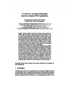
Figure 2: Height field samples are defined at the corners of a regular grid (left), four corner points define a bilinear patch of the height field (middle), the highest resolution mipmap contains the maximumvalue of the bilinear patch (right).

2 Related Work Ray-height field intersection is a pervasive tool in graphics algorithms. The classical application of direct height field rendering is terrain rendering. Terrain rendering is usually performed using level-of-detail techniques that analyze the height field data in an online or offline step and compute an optimized triangulation which is then ray-traced or rendered by rasterization-based approaches, e.g. [Lindstrom et al. 1996; Roettger et al. 1998; Hoppe 1998]. Direct ray tracing of height fields is often based on 2D rasterization [Musgrave 1988; Cohen and Shaked 1993; Cohen-Or et al. 1996; Qu et al. 2003; Henning and Stephenson 2004]. The ray’s projection into the texture domain is rasterized and the cells corresponding to height map pixels are checked for intersections. These algorithms use different acceleration methods. Cohen and Shaked [1993] use a pyramidal data stucture to perform hierarchical ray tracing. Cohen-Or et al. [1996] use an incremental uniform traversal where each pixel column of an image is traced incrementally. Whereas the previous methods use a constant height approximation inside a height field cell, Qu et al. [2003] use different primitives, i.e. planes or polygonal approximations, yielding higher quality renderings for low resolution height fields. Henning and Stephenson [2004] use the run-length’s of the discretized lines to intersect larger bounding volumes with the height field data. Smits et al. [2000] directly intersect displacement mapped triangles using barycentric coordinate hierarchies instead of regular sampling on a two-dimensional grid. In GPU-based real-time rendering algorithms these ray-tracing methods have not become popular. Instead, approximate methods like uniform stepping combined with binary search are dominantly being used [Oliveira and Policarpo 2005; Policarpo and Oliveira 2006]. Alternatively, Newton iterations [Ohbuchi 2003; Wyman 2005; Hu and Qin 2007] or the secant method [Risser et al. 2005; Szirmay-Kalos et al. 2005] are performed either by themselves or combined with uniform search. The former approach is usually being taken when accuracy is not too much of an issue, like in refraction rendering or nearby geometry lookup after refraction or reflection, or when the height map is simple. In case correct intersections are required, intersection methods based on safety zones are being used, e.g. [Donnelly 2005; Baboud and Decoret 2006; Jeschke et al. 2007]. All safety zone techniques known today require off-line pre-computation of the acceleration structure. Donnelly [2005] uses distance maps which require a 3D texture and significant pre-computation times. The memory requirements prohibit the use of this method to render large scale height fields. Lately, methods have been devised that store the safety region information in a 2D texture. Kolb and Rezk-Salama [2005] use multi-channel dilation and erosion maps to define safety regions for empty space skipping. Baboud and Decoret [2006] compute the minimum radius around each height field cell where any ray intersects the surface only once. In stopping the ray traversal this way, one point above and one point below the surface have been found and a binary search is performed to re-

fine the result. Dummer [2006] uses cone ratios to define empty space regions. Policarpo and Oliveira [2007] improve this method by allowing exactly one ray-height field intersection for any ray inside the cone. Again, a binary search follows the ray traversal to refine the result. In contrast to recent GPU-based ray-height field intersection methods we propose to borrow from the earlier CPU-based accurate ray tracing methods to perform scalable and efficient height field intersections. The maximum mipmap is a data structure equivalent to a fully sub-divided quad-tree [Samet 1990] and thus allows for hierarchical traversal of the height map which in practice results in near logarithmic traversal complexity. Minimum-Maximum Mipmaps have been used lately for soft shadow rendering [Guennebaud et al. 2006] and geometry image intersection [Carr et al. 2006]. Guennebaud et al. [2006] use a hierarchical mipmap structure to efficiently determine the occluded region between a point and an area light source. Carr et al. [2006] use minimum-maximum mipmaps to define a hierarchy of axis-aligned bounding boxes for deforming triangle meshes. Once the lowest mipmap level is reached they perform ray-triangle intersections. Our algorithm is mainly inspired by the work of Cohen and Shaked [1993], who use discrete line traversal of a quad-tree to render height fields on a parallel computer, whereas we employ current graphics hardware and a parametric line description. We also use parametric surface patches for the description of a height field within one voxel, whereas [Cohen and Shaked 1993] assume a piecewise constant height field. A similar approach as taken in this paper is presented by Oh et al. [2006]. However, their work has several shortcomings which we improve upon. The major improvements are a truly hierarchical traversal of the maximum mipmap data structure, a viewdependent, adaptive, per-pixel level-of-detail selection and an accurate bilinear patch intersection at the lowest level of the mipmap.

3

Algorithm

Our ray-height-field intersection algorithm is based on an acceleration data structure, the maximum mipmap. This data structure is fast to pre-compute and allows for efficient empty space skipping. In using a mipmap-like data structure for empty-space skipping we balance the complexity of pre-computing the acceleration data structure with that of the ray traversal phase. The maximum mipmap represents an implicit bounding volume hierarchy (BVH) of successively larger cuboids. It is similar to a fully subdivided quad-tree [Samet 1990] storing the maximum heights above the base plane of the height field. Instead of storing parent-child relations as pointers we compute the information onthe-fly. During the ray traversal phase we move the ray position from cell boundary to cell boundary until the ray falls below the height field surface. While moving through the height field hierarchy, we dynamically change the hierarchy level. In case the closest intersection in the forward direction of the ray falls below the height field

Figure 3: During the pre-computation step the maximum value of each cell of the height field is computed. The mipmap data structure is build up by computing the maximum value of the four underlying samples. At the finest level, i.e. level 0, the heights of the four corners of a bilinear patch are stored in one RGBA value.

data the hierarchy level is decreased by one and the intersection computation is repeated until a cell can be passed or the intersection point with the height field surface has been found on the lowest level of the hierarchy. A more detailed description of the intersection algorithm is presented in Sect. 3.2. The intersection computations, i.e. ray-plane intersections for the bounding volumes and ray-bilinear patch (bipatch) intersections for the finest resolution level of the height map, are performed algebraically. A substitution of the analytical ray bilinear patch intersection in the finest mipmap level with an iterative search of the intersection point (i.e. uniform stepping with consecutive binary search) results in increased performance. A comparison between analytical and iterative bilinear patch intersection is presented in Sect. 3.4. In the following we will detail the structure of maximum mipmaps, explain the intersection algorithm in detail and show how to implement level-of-detail rendering using the proposed data structure. Finally, we propose a different data layout to improve the memory access pattern. This results in increased performance due to better cache utilization on current graphics hardware. 3.1 Data Structure

We define the height field as a collection of bilinear patches with data points given at the corner points of a regular grid, see Fig. 2. For convenient access using only one texture fetch, we store the four height values of a bilinear patch in a RGBA texture. For each of the patches we compute the maximum value of the four corner points and store it in the highest resolution mipmap. Afterwards, the mipmap generation process is run. For each coarser level of the mipmap, the maximum height value of the four underlying mipmap pixels is computed. The resulting patch hierarchy is shown in Fig. 3. The mipmap hierarchy can be computed dynamically on the GPU. The following timings have been produced with a Dual Core Opteron 2.6 GHz, equiped with a Geforce 8800 Ultra. As a comparison the timings for the pre-computation of a relaxed cone step map [Policarpo and Oliveira 2007] and a distance map [Donnelly 2005] are provided. All timings use the height field shown in Fig. 6.

2562 5122 10242 20482 40962

maximum mipmap 0.17ms 0.27ms 1.20ms 2.13ms 7.52ms

relaxed CSM ∼ 2 min ∼ 15 min ≥ 8 hours n.a. n.a.

distance maps ∼ 10 sec ∼ 1:20 min ≥ 12 min n.a. n.a.

Table 1: Time needed to pre-compute the acceleration data structures of maximum mipmaps, relaxed cone step mapping (CSM) and distance maps. The z resolution of the 3D distance map is chosen to be one fourth of the x resolution (e.g. 256x256x64).

The table shows that the computation of the acceleration data structure for our maximum mipmaps algorithm is negligibly fast while other state-of-the-art algorithms require considerable precomputation times. The maximum mipmap can be computed onthe-fly providing support for dynamic height fields. 3.2 Intersection Algorithm

The intersection algorithm starts by rendering the bounding geometry of the height map. For each pixel covered by the bounding geometry we cast a ray into the scene, starting at the bounding volume of the height field. traverse_ray: while( ray_above_height_field ) height = sample_maximum_height ( pos, dir, level ); if ( level == 0 && ray_height height || level == 0 ) move_to_intersection_point; update_mipmap_level; else descend_one_mipmap_level; end end Algorithm 1: Ray-height field intersection We start the intersection computation at the highest mipmap level. The main loop of our algorithm then consists of intersecting the bounding planes defined by the mipmap pixel at the current mipmap level. We intersect the four planes bounding the volume on the sides and the plane of maximum elevation. The plane equations are computed on-the-fly from the mipmap sample position. Since we are mainly moving from cell boundary to cell boundary, care has to be taken when determing the sampling position. An important feature of our algorithm is the sampling of the height map at integer positions in the direction of the viewing ray. This measure results in accurately intersected bounding planes even at the corners of a height map pixel. In comparison, Oh et al. [2006] use a small offset vector and sample at non-integer positions which could result in missed intersections. Note that we intersect the plane of maximum elevation as well as the bounding planes of a pixel. This measure lets us determine

Figure 4: Two cases where traversing the hierarchical data structure without ascending steps results in significant performance loss. (left) A height field is observed at a grazing angle. Our algorithm renders the scene at 24 fps, while the algorithm of Oh et al. [2006] achieves only 9 fps. The screen resolution is 800 × 600, the height field resolution is 40962 . (right) With increasing depth of the displacement rendering becomes significantly slower using the algorithm of Oh et al. (27fps). Our algorithm renders this scene at 80 fps. The screen resolution is 800 × 600, height field resolution is 10242 .

whether we can move the ray position forward independent of the intersection result. We can move the ray to the computed intersection point if its current height is above the maximum height of the underlying mipmap cell because the closest intersection point will be at the boundary or at the plane of maximum elevation. In case the ray position cannot be updated because the current mipmap cell is potentially blocking it, we refine the search by descending one level into the hierarchy. At the lowest level, i.e. at the bilinear patch level, the maximum height is determined from the four corner points of the bilinear patch. There are two cases with highly different computational costs to consider. In comparison to an intersection with the bounding planes of a mipmap pixel, a bilinear patch intersection is expensive to compute. Therefore, we only perform the bilinear patch intersection if a potential intersection exists. After moving the ray position, we perform an update of the current mipmap level. The necessity for this update arises when a ray passes very close to the height field surface but does not intersect it. The algorithm potentially descends to the bilinear patch level of the mipmap hierarchy to determine that an intersection does not take place. Without ascending again, the algorithm would be forced to take very small steps for potentially a large number of iterations until the ray finally hits the surface or leaves the bounding volume of the height field. There are different strategies to perform the update of the hierarchy level. Depending on the cell boundary at the current ray position, the algorithm can jump into different levels of the bounding volume hierarchy represented by the maximum mipmap. However, the online computation of this information requires a loop with a dynamic stopping condition. Current graphics hardware is not well suited to this kind of computation. Alternatively, the information can be stored in an additional texture. However, accessing this texture results in performance loss similar to the dynamic loop. We found that the most performant update strategy is to simply increase the mipmap level by one in case the ray resides at a cell boundary divisible by two. The disadvantage of ascending only one hierarchy level is compensated by faster computation and simpler algorithmic structure. In comparison to our method Oh et al. [2006] do not ascend in the hierarchical data structure, therefore not taking complete advantage of the empty space skipping capabilities of the maximum mipmap. Thus, in case no intersection is found their algorithm is forced to take very small steps once the lowest hierarchy level is reached, effectively resulting in a linear search. This has considerable performance drawbacks at grazing angles and when rendering displacement maps with high depth complexity, see Fig. 4.

Figure 5: During the ray propagation phase a mipmap hierarchy structure is used to perform empty space skipping. The figure shows a path through the mipmap data structure for a given height field. The curve at the bottom represents a one-dimensional height field consisting of linear elements at the lowest level. The tree on the top symbolizes the maximum mipmap. Each cell contains the maximum value of the height field within that cell. The black line shows the order of traversal chosen by our algorithm.

In Fig. 5 we show a one-dimensional example of ray-height field intersection using the proposed algorithm. The figure shows a fully subdivided quad-tree containing the maximum height field values for its nodes’ bounding volumes. At the bottom, a one-dimensional height field consisting of linear elements and a ray are depicted. The thick black line shows the traversal order chosen by our algorithm. The first six steps require the algorithm to descend to level 1 of the bounding volume hierarchy to pass the “hill” in cell 4 and 5. Afterwards, successively larger steps can be taken until a parent of cell 12 containing the correct intersection is found. The algorithm then again descends into the hierarchy, computing the correct intersection point. In comparison to other ray-height map intersection algorithms, e.g. uniform stepping with binary search [Oliveira and Policarpo 2005; Policarpo and Oliveira 2006], our algorithm requires less iteration steps until a correct intersection point is found. The number of steps is comparable to other pre-computation based techniques like relaxed cone step mapping [Policarpo and Oliveira 2007]. Unfortunately, the performed steps are more complex, since a hierarchical data structure is being used. Fig. 8 shows the number of iteration steps required to find the correct intersection point of the ray and the height field. A performance comparison of different algorithms is given in Sect. 4. 3.3 Level of Detail

The main advantage of using maximum mipmaps as acceleration data structure is the possibility of getting level of detail rendering capabilities almost for free. Based on the distance between the camera and the intersection point the maximum level of the mipmap that still projects to less than one pixel on screen can adaptively be determined and subtrees of the bounding volume hierarchy can be pruned. Hence to support height map mipmapping we change algorithm 1 slightly to yield algorithm 2. The potential slow down of using additional variables and instructions is low in comparison to the speed up we achieve by stopping the ray propagation earlier. The formulation of our switch_lod function is modeled after the following observation. Since the area of space covered by one pixel changes linearly with respect to the depth of the ray position in eye space, it can be used to define a simple Level-of-Detail function. Before running the height field intersection shader, we determine the distance at which one height field pixel on the base plane projects to one pixel on the screen. This value is stored in the dis-

Figure 6: Test scene used for the comparison of the performance of different algorithms. Note how detail increases with higher resolution. Height map resolution from left to right: 10242 , 20482 and 40962 . For the resolutions 2562 and 5122 the height map 10242 was scaled down. traverse_ray:

compute the correct intersection point of a ray with a height field cell on the lowest hierarchy level an intersection with a bilinear patch has to be computed. Ramsey et al. [2004] show an analytical solution of the ray-bilinear patch intersection problem, which we height = sample_maximum_height implement. Unfortunately the computation costs of such an inter( pos, dir, level ); section on the GPU are high due to the strong branching structure of the algorithm and the performance decreases considerably. if( switch_lod( pos, height, lod ) ) lod++; An alternative solution is to use uniform stepping combined with binary search [Policarpo et al. 2005] to intersect the ray with the biif ( level == 0 && ray_height height || level == lod ) Oh et al. [2006] propose another method for finding the final move_to_intersection_point; intersection of the ray with a bilinearly interpolated heightmap cell. update_mipmap_level; They perform a linear approximation of the quadratic height field else profile along the viewing ray. This results in artifacts where the descend_one_mipmap_level; bilinearly interpolated height field does not behave approximately end linear. Furthermore, they do not check against the boundaries of the bilinear height field patch, potentially generating intersections level = max( level, lod ); outside the support of the patch. A visual example of the artifacts introduced by their algorithm is shown in Fig. 7. end Table 3 shows frame rates achieved by using the maximum mipmap algorithm without bilinear patch intersection, using the anAlgorithm 2: Ray-height field intersection with Level of Detail alytical approach and when performing an iterative search to determine the ray-bilinear patch intersection. while( ray_above_height_field )

tance_factor variable. At double the distance, a patch of four time the area will project to one pixel. However, since the height field defines elevation values, a cell could still contain a large spike and project to multiple pixels on the screen, resulting in visible artifacts. To prevent these, we subtract the maximum value of the current height field cell from the ray’s z-coordinate and clamp the result to zero. max((ray_depth − height) − 2lod ∗ distance_ f actor, 0) > 0. Using this conservative heuristic results in artifact-free rendering in most of the cases. Additionally, as suggested by [Tatarchuk 2006], we could switch to simple bump mapping [Blinn 1978] once the distance to the displacement mapped surface becomes large. However, we do not currently implement this. 3.4 Performance Improvements

In comparison to other algorithms the algorithm presented in this paper cannot take advantage of hardware interpolation. Hence to

2562 5122 10242 20482 40962

maximum mipmap 95 87 75 70 49

+ bilinear patch intersection 43 38 33 27 22

+ linear binary search 70 58 50 40 35

Table 3: Performance (in frames per second) of the maximum mipmap algorithm. The first column shows timings without bilinear patch intersection. The second and the third column show results using analytical ray-bilinear patch intersection and uniform combined with binary search, respectively. The rendering is performed at a screen resolution of 1024 × 768 pixels. The iterative search uses 10 linear and 6 binary search steps. Additional speed-ups can be achieved by re-arranging the mipmap information in graphics memory. Due to the hierarchical structure of our algorithm the memory access pattern is incoher-

2562 5122 10242 20482 40962 Figure 7: A height field with several saddles rendered using our bilinear patch intersection (left) and using the method proposed by Oh et al. [2006] (right).

640x480 800x600 1024x768 1200x900

uniform + binary 120 86 56 43

relaxed CSM 390 310 227 182

maximum mipmap 154 110 75 57

MM + LOD 189 140 90 69

Table 4: Performance (in frames per second) of different algorithms for different screen resolutions, height map resolution is 10242 . The number of linear search steps for the first algorithm is empirically chosen to yield the same rendering quality as the maximum mipmap algorithm and to assure temporal coherence. Test scene is shown in Fig. 6

ent, thus resulting in cache misses. Although graphics hardware is highly optimized for mipmap accesses the frequent switches between hierarchy levels in our algorithm seem not to be well supported by todays GPUs. Our experiments show that cache misses can be significantly reduced by storing the mipmap information in continuous texture locations. This can be done by storing the mipmap data into a 3D texture. The depth slices then contain all mipmap levels at a particular 2D texture location. We observed speed-ups of 15 − 20% when using this memory layout. However, the memory requirements are considerable. Please note, that the timings provided in the next section do not include this optimization.

4 Comparison We compare our maximum mipmap algorithm against representative algorithms from the two classes of height field intersection algorithms, approximate methods for dynamic height fields and algorithms based on pre-computed acceleration data structures for static height fields. The observations equally apply to the method of Oh et al. [2006] in most of the cases, the drawbacks of which have already been discussed in the previous sections. As a representative of the class of approximate intersection methods, requiring no pre-computation, we choose linear stepping combined with binary search [Policarpo and Oliveira 2006]. The alternatives such as Newton iterations [Ohbuchi 2003; Wyman 2005; Hu and Qin 2007] or the secant method [Risser et al. 2005; Szirmay-Kalos et al. 2005] are only suitable for simple height maps when employed by themselves. In combination with uniform search the uniform part of the resulting algorithm dominates the computation costs by far, justifying our restriction to only one algorithm. The class of accurate intersection algorithms requiring precomputation is represented by the relaxed CSM algorithm [Policarpo and Oliveira 2007]. Our choice is motivated by the ability of the CSM algorithm to store the acceleration data structure in a 2D texture. Distance maps are excluded because of too high memory requirements. The results of two performance tests are shown in tables 4 and 5.

uniform + binary 150 103 56 32 9

relaxed CSM 240 233 227 n.a. n.a.

maximum mipmap 95 87 75 70 49

maximum mipmap + LOD 110 102 90 89 77

Table 5: Performance of different algorithms for different height map resolutions, screen resolution is 1024 × 768. Maximum mipmaps scale well with increasing height field resolution, whereas the combination of uniform and binary search becomes inefficient for large maps. CSM timings for height map resolutions larger than 10242 cannot be provided due to impractically large precomputation times. Test scene is shown in Fig. 6

The first test, table 4, shows the dependence of the rendering performance on the screen resolution. In the second test we investigate the impact of the height field resolution on the rendering performance. The first test, table 4, shows a near linear dependency of all algorithms on the screen resolution. This is expected since all algorithms are ray casting variants, their run-time depending on the number of affected pixels. In the second test, table 5, we show that the maximum mipmap algorithm outperforms algorithms based on uniform search for height maps larger than 5122 . This number can vary, depending on the height field structure. In the accompanying video we show additional examples. Usually the trade-off point between the two algorithms is somewhere between the resolutions of 5122 and 10242 . The CSM algorithm generally performs faster than both uniform search and maximum mipmaps. However, because of the large precomputation times it is only suitable for use with static height maps. In a third test, we show the accuracy of the three algorithms in our test. Fig. 9 shows that maximum mipmaps produce artifact-free renderings while algorithms based on uniform search show considerable artifacts at the same rendering frame rate for a height map of 10242 . This behavior is getting worse with increased height map resolution. Relaxed cone step mapping on the other hand should be nearly artifact-free, however, our results, using the implementation of Policarpo and Oliveira [2007], also show problems with very narrow height field structures. Please note that the spiky appearance of the height map is due to grayscale anti-aliasing in the image processing tool that was used for the generation of our height maps. An additional advantage of the maximum mipmap algorithm is that artifact-free renderings can be produced without parameter adjustments. Algorithms using uniform stepping require proper adjustments on the number of iteration steps for every height map to achieve artifact-free results. Furthermore, the maximum mipmap algorithm exhibits more stable rendering frame rates when different parts of the height map are rendered or different gazing angles are being used.

5

Results

We have implemented the technique described in this paper as a Shader Model 4.0 fragment program. The timings and the accompanying video were produced using a Dual Core Opteron 2.6 GHz, equiped with a Geforce 8800 Ultra. For the results shown in the video we have implemented tangent space relief mapping [Policarpo et al. 2005] as an example application. In the video we first show a comparison between the proposed algorithm and uniform combined with binary search as well as relaxed cone step mapping. Our algorithm accurately renders very narrow structures of the height fields whereas the other algorithms produce artifacts. Next we demonstrate the scalability of our algorithm by render-

Figure 8: Number of steps performed until the ray hits the height field, maximum mipmaps (left), linear + binary search (middle), relaxed cone stepping (right). The resolution of the height field is 10242 .

ing a highly complex height field in the venus scene. The highest resolution height field (40962 ) can still be rendered at interactive frame rates while the algorithm based on uniform search achieves only ≈ 4 fps. It was not possible to produce equivalent results for the relaxed CSM algorithm due to the large pre-computation times. Please note that the height field is rendered twice to support reflection in the pool of water below the statue. To demonstrate the feasibility of large scale dynamic height field rendering we blur the height field of the statue in real time using a gaussian filter kernel. This gives an effect of the statue melting into the background brick wall. Note that this is not possible with other accurate state-of-the-art algorithms. Throughout the video, the maximum mipmap algorithm is executed with Level of Detail rendering and bilinear patch intersections. The bilinear patch intersections have been computed using the iterative search method proposed in Sect. 3.4. The video has been rendered at a constant frame rate of 25 frames per second, the timings given in the video are taken from a corresponding rendering session at a resolution of 800 × 600 pixels. The final video has been scaled down to 640 × 480 pixels.

6 Conclusions We have presented a fast and accurate height field intersection technique based on a hierarchical data structure, the maximum mipmap. The algorithm scales well to large scale height fields and shows favorable performance for medium to large scale maps compared against approximate intersection techniques. In comparison to other algorithms based on pre-computed data structures the maximum mipmap is very fast to update, requiring only one mipmap update. This enables the use of our algorithm for real-time dynamic height field rendering. The ability to use Level of Detail rendering is inherent in our algorithm and contributes to the performance observed for large scale height fields. We therefore think that our algorithm presents a valuable contribution for real-time algorithms that rely on efficient and accurate ray-height field intersections. For future work we would like to consider provably correct Level of Detail selection techniques. Additional work includes the efficient use of Level of Detail techniques for efficient height field shadow mapping and its application in the tangent space of objects. Another possibility is the investigation of hierarchical height field rendering techniques in shell space [Porumbescu et al. 2005; Jeschke et al. 2007] and the use of different hierarchy representations such as barycentric hierarchies [Smits et al. 2000].

References BABOUD , L., AND D ECORET, X. 2006. Rendering Geometry with Relief Textures. In Proceedings of Graphics Interface 2006, 195–201. B LINN , J. 1978. Simulation of Wrinkled Surfaces. In Proceedings of SIGGRAPH’78, 286–292.

C ARR , N. A., H OBEROCK , J., C RANE , K., AND H ART, J. C. 2006. Fast GPU Ray Tracing of Dynamic Meshes using Geometry Images. In GI ’06: Proceedings of Graphics Interface 2006, 203–209. C OHEN , D., AND S HAKED , A. 1993. Photo-Realistic Imaging of Digital Terrains. Computer Graphics Forum 12, 3, 363–373. C OHEN -O R , D., R ICH , E., , L ERNER , U., AND S HENKAR , V. 1996. A Real-Time Photo-Realistic Visual Flythrough. IEEE Transactions on Visualization and Computer Graphics 2, 3, 255– 265. C OOK , R. L. 1984. Shade Trees. GRAPH’84, 223–231.

In Proceedings of SIG-

D ONNELLY, W. 2005. GPU Gems 2. Addison-Wesley Professional, ch. Per-Pixel Displacement Mapping with Distance Functions. D UMMER , J., 2006. Cone Step Mapping: An Iterative Ray-Heightfield Intersection Algorithm. http://www.lonesock.net/files/ConeStepMapping.pdf. G UENNEBAUD , G., BARTHE , L., AND PAULIN , M. 2006. RealTime Soft Shadow Mapping by Backprojection. In Proceedings of EGSR’06, 227–234. H ENNING , C., AND S TEPHENSON , P. 2004. Accelerating the Ray Tracing of Height Fields. In Proceedings of the 2nd international conference on Computer graphics and interactive techniques in Australasia and South East Asia, 254–258. H OPPE , H. 1998. Smooth View-Dependent Level-of-Detail Control and its Application to Terrain Rendering. In VIS ’98: Proceedings of the conference on Visualization ’98, 35–42. H U , W., AND Q IN , K. 2007. Interactive Approximate Rendering of Reflections, Refractions, and Caustics. IEEE Transactions on Visualization and Computer Graphics 13, 1, 46–57. J ESCHKE , S., M ANTLER , S., AND W IMMER , M. 2007. Interactive Smooth and Curved Shell Mapping. In Proceedings of EGSR’07, 351–360. KOLB , A., AND R EZK -S ALAMA , C. 2005. Efficient Empty Space Skipping for Per-Pixel Displacement Mapping. In Proceedings of Vision, Modeling and Visualization (VMV’05), 407–414. L INDSTROM , P., KOLLER , D., R IBARSKY, W., H ODGES , L. F., FAUST, N., AND T URNER , G. A. 1996. Real-time, continuous level of detail rendering of height fields. In Proceedings of SIGGRAPH’96, 109–118.

M USGRAVE , F. K. 1988. Grid Tracing: Fast Ray Tracing for Height Fields. Tech. Rep. YALEU/DCS/RR-639, Yale University, Dept. of Computer Science Research. O H , K., K I , H., AND L EE , C.-H. 2006. Pyramidal Displacement Mapping: a GPU based Artifacts-Free Ray Tracing through an Image Pyramid. In VRST ’06: Proceedings of the ACM symposium on Virtual reality software and technology, 75–82. O HBUCHI , E. 2003. A Real-Time Refraction Renderer for Volume Objects Using a Polygon-Rendering Scheme. In Proceedings of Computer Graphics International, 190–195. O LIVEIRA , M. M., AND P OLICARPO , F. 2005. An Efficient Representation for Surface Details. Tech. rep., Universidade Federal do Rio Grande do Sul. P OLICARPO , F., AND O LIVEIRA , M. M. 2006. Relief Mapping of Non-Height-Field Surface Details. In Proceedings of I3D’06, ACM Press, 55–62. P OLICARPO , F., AND O LIVEIRA , M. M. 2007. GPU Gems 3. Addison-Wesley Professional, ch. Relaxed Cone Stepping for Relief Mapping. P OLICARPO , F., O LIVEIRA , M. M., AND C OMBA , J. L. D. 2005. Real-Time Relief Mapping on Arbitrary Polygonal Surfaces. In Proceedings of I3D’05, 155–162. P ORUMBESCU , S. D., B UDGE , B., F ENG , L., AND J OY, K. I. 2005. Shell Maps. In Proceedings of SIGGRAPH’05, 626–633. Q U , H., Q IU , F., Z HANG , N., K AUFMAN , A., AND WAN , M. 2003. Ray Tracing Height Fields. In Proceedings of Computer Graphics International, 9-11, 202–207. R AMSEY, S. D., P OTTER , K., AND H ANSEN , C. 2004. Ray Bilinear Patch Intersections. Journal of Graphics Tools 9, 3, 41–47. R ISSER , E., S HAH , M., AND PATTANAIK , S. 2005. Interval Mapping. Tech. rep., University of Central Florida. ROETTGER , S., H EIDRICH , W., AND S LUSSALLEK , P. 1998. Real–Time Generation of Continuous Levels of Detail for Height Fields. In Proc. 6th Int. Conf. in Central Europe on Computer Graphics and Visualization, 315–322. S AMET, H. 1990. The Design and Implementation of Spatial Data Structures. Addison - Wesley Publishing Company Inc. S MITS , B., S HIRLEY, P., AND S TARK , M. 2000. Direct Ray Tracing of Smoothed and Displacement Mapped Triangles. PhD thesis. S ZIRMAY-K ALOS , L., A SZODI , B., L AZANYI , I., AND P RE MECZ , M. 2005. Approximate Ray-Tracing on the GPU with Distance Impostors. Computer Graphics Forum 24, 3 (Sept.), 695–704. TATARCHUK , N. 2006. Dynamic Parallax Occlusion Mapping with Approximate Soft Shadows. In I3D ’06: Proceedings of the 2006 symposium on Interactive 3D graphics and games, 63–69. W YMAN , C. 2005. Interactive Image-Space Refraction of Nearby Geometry. In Proceedings of the 3rd international conference on Computer graphics and interactive techniques in Australasia and South East Asia, 205–211.

Figure 9: Rendering quality of different algorithms, renderings performed at the same frame rate. Maximum mipmaps (top), linear + binary search (center), relaxed cone stepping (bottom). The resolution of the height field is 10242 . The frame rate is 27 FPS (for maximum mipmaps and linear binary search). The sharp spikes are produced by antialiased font rendering into the height field. Note that relaxed CSM and linear + binary search can miss thin structures, whereas maximum mipmaps render thin structures correctly.