Modeling of Cyclist Acceleration Behavior Using Naturalistic GPS Data Ding Luo and Xiaoliang Ma*
Traffic Simulation & Control (TSCLab), Division of Transport Planning, Economics and Engineering (TEE), Department of Transport Science, KTH Royal Institute of Technology Teknikringen 10, Stockholm 10044, Sweden * Corresponding author:
[email protected]
Submitted for presentation at the 95th Transportation Research Board Annual Meeting, 2016 5070 words + 2 Table (2 X 250) + 5 Figures (5 X 250) = 6820 words + 22 References
2 Ding Luo and Xiaoliang Ma
Abstract 1 2 3 4 5 6 7 8 9 10 11 12 13 14 15 16 17 18
Cycling is a healthy and sustainable mode of transportation. However, various problems, such as bicycle congestion, cycling safety and accessibility issues have been frequently observed in cities like Stockholm due to the rapidly increasing number of cyclists and insufficient bicycle facilities. In comparison to the overwhelming research effort on vehicle traffic and driver behavior, the studies on bicycle movement and cyclist behavior are however still far behind. This paper therefore aims at bridging the gap by presenting a new methodology for investigating and modeling microscopic cyclist behavior. In particular, the paper focuses on representing bicycle movements when they are not interacting with others. The cyclist acceleration behavior is modeled using naturalistic GPS (Global Positioning System) data collected by eleven recruited commuter cyclists from Stockholm. After processing the large amount data, cyclist trajectories are obtained and acceleration profiles are selected. A mathematical model is proposed and then identified by the acceleration datasets using the maximum likelihood estimation methodology. The cross validation approach is conducted to compare different forms of the mathematical model. While the model with more parameters shows superior performance, the simplified ones are still capable of capturing the trends in the acceleration profiles. Moreover, model extension is also discussed to show the possibility of examining the impact of cyclist specific factors, such as age, gender and agility, on cyclist behavior by using the proposed model. Although the cyclist population investigated in the current study is still limited, it is believed that our research provides a unique insight into this non-motorized transportation mode and could promote future bicycle related studies.
3 Ding Luo and Xiaoliang Ma 1
1. INTRODUCTION
2 3 4 5 6 7 8 9 10
Many cities in Europe and US have witnessed the growing cyclist population over the past decades. Although the size of this community is still small in comparison to motorized vehicles, increasing attention has been given to its high level of vulnerability in traffic safety research. In the meantime, a tremendous demand for more knowledge of the characteristics specific to this traveler group has also been identified provided with the new policy trend for sustainable transport development (1). As the popularity of cycling increases at a fast pace in most urban areas, both traffic planners and policy makers have been seeking useful analytical tools which can effectively facilitate addressing bicycle related planning and operational issues. Since the development of these tools, such as the bicycle traffic simulation models, highly depends on sufficient understanding of cyclist behavior, it becomes even more urgent for researchers to advance in that direction.
11
1.1 Relevant studies
12 13 14 15 16 17 18 19 20 21 22 23 24 25 26 27 28 29 30 31 32 33 34 35 36 37 38 39 40 41 42 43 44 45 46 47 48 49 50 51 52 53 54
Although the significance of bicycle as one of the most convenient and environmentally friendly non-motorized transport modes has been highlighted by many studies, there is still a considerable gap in the current literature compared to fruitful results of vehicular traffic flow and driver behavior. A consensus has been achieved by many researchers that bicycle traffic differs remarkably from the vehicular one and exclusive research on cyclist behavior is of great necessity. Two facts that cause the difference are suggested by Twaddle et al. in (2), i.e. the dynamic characteristics of cyclists, including their speed, acceleration and deceleration profiles, and the physical characteristics, including size, flexibility and capability. Moreover, Twaddle et al. in (2) reviewed existing studies on modeling cyclist behavior and summarized the state of the art in the modeling approaches. They categorized all the models into four groups: longitudinally continuous models, CA (Cellular Automata) models, social force models and logic models. In addition, an assessment on the ability of realistically modeling bicycle traffic on four levels was also performed, including uninfluenced operational, uninfluenced tactical, influenced operational, and influenced tactical levels. Despite the insufficiency of research on the modeling of cyclist behavior, an increasing number of studies on modeling mixed traffic can be seen in the literature. For instance, Oketch (3) presented a new method for modeling mixed-traffic streams which allows the inclusion of many different kinds of transportation modes, such as motorcycles, bicycles, three-wheeled vehicles and even pedestrian pulled carts. Schönauer et al. (4) attempted to model the social behavior of cars, pedestrians, and bicycles in the interactions by adopting a social force model. Manar et al. (5) presents a comparison of a set of six bike-following models. Gould et al. (6) tried to derive the macroscopic properties of bicycles using CA, while Zhao et al. (7) attempted to model passing events in mixed bicycle traffic with CA. Experiences from research on motorized vehicles indicate that the availability of sufficient field data, or naturalistic data is extremely important to the understanding and modeling of cyclist behavior. Given the demand for high quality data, the Instrumented Probe Bicycle (IPB) emerged as an attractive and reliable tool. Although currently there is no standardization of IPB, this technology is developing rapidly and many researchers have successfully carried out bicycle related studies using data collected by different IPBs. In the beginning the IPB was quite basic with a few types of equipment mounted and most of those studies merely aimed at investigating the cyclist behavior on a relatively macroscopic level, such as identifying the risk factors existed in the bicycle activities and obtaining cycling routes and speed distributions, see (8, 9, 10, 11). Most recently, however, more developed IPBs became available and deeper insight into bicycle mobility was presented. For instance, Joo et al. (12) employed an IPB equipped with a set of sensors including a GPS receiver, an accelerometer, and a gyro sensor. According to their report, good quality data for identifying longitudinal, lateral, and vertical maneuverings of bicycle movement could be obtained from the IPB. Consequently, an intelligent system called Bicycle Monitoring Index (BMI) which can be used to evaluate the safety and mobility of the bicycle environment was developed using the fault tree analysis (FTA) technique. Dozza et al. (13) designed an even more advanced IPB with multiple sensors to study bicycle dynamics and cyclist behavior. Longitudinal, lateral, and vertical accelerations were measured and further processed by specialized software. It was concluded that high quality naturalistic data from the IPB laid a solid foundation for further development of bicycle related applications. Furthermore, some researchers attempted to study cyclists’ performance at intersections since it was pointed out that vehicle-bicycle collisions occurred at intersections are the most common issues due to the insufficient clearance time for cyclists traveling at their ordinary cruising speed (14). Pein in (15) investigated cyclist performance both on multiuse trails and at three-leg intersections. The study found that the cyclists did not accelerate uniformly, with the acceleration rate decreasing after an initial increase. Nevertheless, the research was not continued and no more detailed results were available. Figliozzi et al. (16) developed a methodology for
4 Ding Luo and Xiaoliang Ma 1 2 3 4
estimating cyclist acceleration and speed distributions at intersections. They employed a basic video setup to collect field data and further presented some statistical analyses on cyclist acceleration and cruising speed performance at intersections. In addition, some studies, e.g. (10), also tried to figure out whether cyclist demographics have an influence on cycling performance and cyclist behavior, yet no consensus so far has been reached.
5
1.2 Objectives and Structure
6 7 8 9 10 11 12 13 14
The main objective of this study is to seek analytical approaches which could improve the understanding of cyclist behavior under common circumstance based on high frequency GPS data, especially for the acceleration and deceleration behaviors. Detailed cycling characteristics are expected from data analysis and modeling work for promoting future research on bicycle movement and cyclist behavior. The remainder of this article is organized as follow: in the second section the data collection and processing are briefly described so that the subsequent modeling part can be better understood by the readers; section 3 shows the main contribution of this study with a methodology for modeling cyclist acceleration behavior. Model identification, validation and extension are presented as well; finally, the research was summarized with conclusions and future work in section 4.
15
2. DATA COLLECTION AND PROCESSING
16
2.1 Data Collection
17 18 19 20 21 22 23 24 25 26 27 28 29 30 31
The data collection was organized twice in Stockholm, respectively in the summer and autumn 2013 and the spring 2014. Eleven commuter cyclists living in Stockholm, three female and eight male, were recruited for the data collection. In the beginning different types of devices were prepared for the data collection, yet practical testing results showed that the Garmin 60CSx and iPhone APP used were not capable of providing high quality data. Therefore neither of them was employed for the data collection and all participants were later provided with handlebar mountable Garmin Edge 500 GPS devices (see FIGURE 1a). All participants were required to record their normal cycling trips as many as possible using the provided devices. Devices were regularly retrieved by the authors in order to upload the data. Eventually, 126 available cycling trips completed in the urban area of Stockholm were sorted out and stored in the database. Several representative cycling trajectories can be viewed in FIGURE 1a. Both applied Garmin devices were able to measure and record GPS data and altitude data with a time interval of one second depending on the high-sensitivity integrated GPS receivers and the internal barometric altimeters, respectively. The GPS data included not only the original measurements of latitude and longitude with eight digits in the fractional part, but also the derived information of distance and speed. Moreover, the altitude data turned out to be relative measurements instead of absolute measurements in most cases due to the limitation of the internal barometric altimeters.
32
2.2 Data Processing
33 34 35 36 37 38 39 40 41 42 43 44 45
While detailed work about data processing has been presented in our previous study (17), only a summary of methodology and results is illustrated in this section so that the following analysis and modeling part can be better understood by the readers. In general, the altitude measurements were smoothed using locally weighted regression (18) and an example of smoothed altitude profile is shown in FIGURE 1b. This processing resulted in more smoothed gradient profiles which were used for subsequent data filtering. As to the GPS data, it was found that missing observations and noise caused by the urban canyon effect undermined the consistency of measurements and further had a non-negligible on data analysis and behavioral modeling. Therefore, signal processing techniques were adopted to solve these issues in our study. After trying some estimation approaches from the simple ARMA (Autoregressive Moving Average) filters to more advanced adaptive filters, the Kalman filter (KF) based approaches finally brought the most consistent estimation results. The KF filter is an advanced method which is able to give optimal estimates of discrete data. The approach was first suggested by Kalman (19) and has been widely used in signal processing and control systems over the past few decades. In this study, using the method allowed us to take advantages of high-frequency GPS measurements. As a result, not only
5 Ding Luo and Xiaoliang Ma
Start End
Garmin Device
(a)
6
22
5
speed (m/s)
20
Altitude (m)
18 16
4 3 2
Observed speed Filtered speed
1 0
14
0
10
20
30
40
50
60
70
40
50
60
70
Time (s) (c)
12
8 6
1 2 3 4 5 6 7 8 9 10 11
Measured altitude Smoothed altitude 0
50
100
150
200 Time (s) (b)
250
300
350
400
acceleration (m/s2)
1
10
0.5 0 -0.5 -1
Derived acceleration 0
10
20
30 Time (s) (d)
FIGURE 1 Illustrations for data collection and processing. Representative cycling trajectories in the urban area of Stockholm (a); An example of the comparison between measured and smoothed altitude profiles (b); An example of the comparison between observed and filtered speed profiles (c); An example of derived acceleration profile (d). was the problem of missing observations addressed by the “Predict” procedure of KF filter, but also the measurement noise was largely removed from the filtering at the same time (see FIGURE 1c). Moreover, the acceleration profiles were obtained as well as shown in FIGURE 1d. The specific implementation of the KF filter referred to a previous study (20) in which the extended Kalman smoothing algorithm was applied to estimate the car-following data collected by an instrumented vehicle.
12
3. MODEL DEVELOPMENT
13
3.1 Cycling Regimes
14 15 16 17 18 19 20 21 22 23 24
While looking through the speed and acceleration datasets, it was found that when significant increases in speed were carried out by the cyclists, the patterns of the change in acceleration rates during the same period showed great similarity regardless of other factors. Specifically, the U-shape acceleration-time profiles were frequently observed together with the S-shape speed-time profiles. Likewise, the same patterns could be observed in the deceleration cases. FIGURE 2a then illustrates a 400-second speed profile example, along with its corresponding acceleration profile. Besides the normal curves, a significant acceleration process and a deceleration process are also marked by red and green dash lines, respectively. Detailed profiles for both acceleration and deceleration cases are further demonstrated in FIGURE 2b and FIGURE 2c, respectively. Apart from those two types of processes which could almost be certainly identified, some processes during which no striking change in speed were also observed with their corresponding acceleration profiles merely exhibiting insignificant fluctuations around zero. In the current study, such processes were labeled as cruising processes. Some examples for each kind of process were shown in
6 Ding Luo and Xiaoliang Ma
speed (m/s)
12 9 6 3 200
250
300
350
400 time (s)
450
500
550
600
250
300
350
400 time (s)
450
500
550
600
acceleration (m/s2)
1 0.5 0 -0.5 -1 200
Identified acceleration process
Identified deceleration process
(a)
10
8
speed (m/s)
speed (m/s)
9 8 7 6 5
Identified cruising process
7 6 5
4 3 250
254
262
0.4 0.2 0 254
258 time (s)
262
observations
(b) 1 2 3 4 5
525
527 529 time (s)
531
533
525
527 529 time (s)
531
533
0
0.6
250
4 523
266
acceleration (m/s2)
acceleration (m/s2)
0.8
258 time (s)
266
-0.2
-0.4
-0.6 523
observations
(c)
FIGURE 2 An illustration of identification of different processes (a); The detail of identified acceleration-‐time and speed-‐time profiles for the acceleration case (b); The detail of identified acceleration-‐time and speed-‐time profiles for the deceleration case (c).
7 Ding Luo and Xiaoliang Ma 1 2 3 4 5 6 7
FIGURE 2a. As a result of our finding, three cycling regimes including acceleration, deceleration and cruising were proposed. Given these three regimes, the cycling behavior can be roughly reflected in a way that a cyclist is always endeavoring to achieve and maintain a desired speed which varies depending on multiple factors, such as the age and gender of the individual (internal factors), and the road grade and weather (external factors). The processes during which the cyclist is maintaining her present desired speed then corresponds to the cruising behavior, while the processes during which he tries to achieve her desired speed refers to either the acceleration behavior or the deceleration behavior. The proposed idea is further summarized as follow:
8
𝑎!"" 𝑡 , 𝑖𝑓 𝑣 𝑡 < 𝑣!"# 𝑎 𝑡 = 𝑎!"# 𝑡 , 𝑖𝑓 𝑣 𝑡 > 𝑣!"# 0, 𝑜𝑡ℎ𝑒𝑟𝑤𝑖𝑠𝑒
(1)
9 10 11 12 13 14 15 16 17 18 19 20 21 22 23 24 25
where 𝑎 𝑡 denotes the acceleration rate at time t; 𝑎!"" 𝑡 and 𝑎!"# 𝑡 , respectively, denote the acceleration rate and deceleration rate at time t; 𝑣!"# denotes the cyclist’s desired speed at time t which could be dependent on a multiple factors. An empirical approach was applied to distinguish significant acceleration or deceleration profiles from the original dataset. Consecutive speed-up and slowing-down data clusters were first identified, followed by a strict filtering based on six criteria shown as follow. The entire filtering process was carried out using MATLAB codes and SQL queries. l The maximum acceleration of a profile 𝑎!"# is smaller than 2 m s ! (or the minimum acceleration 𝑎!"# is larger than −2 m s ! for the deceleration case); l The final speed of a profile 𝑣! is smaller than 15 m s (or the initial speed 𝑣! is lower than 15 m/s for the deceleration case); l The acceleration time of a profile 𝑡! is between 5 seconds and 16 seconds; l The total distance during the acceleration process 𝑑! is not shorter than 5 meters; l The road gradient over the entire acceleration process 𝑔! is neither greater than 10% nor smaller than
26
𝜏=
27 28 29 30 31 32 33 34 35
where 𝑣! and 𝑣! , respectively, denote the initial speed and final speed of a process. As a result, 831 acceleration profiles (8005 observations) and 704 deceleration profiles (5559 observations) respectively stood out. Analysis on these profiles then revealed some characteristics of acceleration and deceleration processes which are in part illustrated in FIGURE 3. Due to the resemblance between the acceleration case and deceleration case, only plots for the former one are presented in the article. It can be seen that in most cases, the variance in speed during the acceleration process lies in a range between 2 m/s and 6 m/s, while the maximum acceleration rate mainly varies between 0.5 m/s2 and 1 m/s2.
−10%;
l
The variance in speed of an acceleration process is significant in a way that the value of a newly defined index 𝜏 should not be lower than 0.5. !! !!!
!"# (!! ,!! )
(2)
8 Ding Luo and Xiaoliang Ma
90
90
Frequency
120
Frequency
120
60 30 0 0 1 2 3 4 5 6 7 8 9 10 Speed difference ΔV (m/s) (a) 1 0.5
120
2
R =0.64 Frequency
lnamax
(b) 150
0 -0.5 -1
90 60 30
-1.5
1 2 3 4 5 6 7 8 9 10 11 12 13 14
30 0 0 0.5 1 1.5 2 2 Maximum acceleration amax (m/s )
lnam ax=0.8248*lnΔ V-1.3263
-2 0
60
0.5
1
1.5 Δ ln V (c)
2
2.5
0 5 6 7 8 9 10 11 12 13 14 15 16 Acceleration time ta (s) (d)
FIGURE 3 Some characteristics of cyclists’ acceleration behavior. (a) Distribution of the variance in speed (∆𝑽); (b) Distribution of the maximum acceleration 𝒂𝒎𝒂𝒙 ; (c) The linear relationship between transformed ∆𝑽 and 𝒂𝒎𝒂𝒙 ; (d) Distribution of the acceleration time 𝒕𝒂 . One important thing that was figured out through data analysis was that the maximum acceleration 𝑎!"# of a process could be, to a large degree, explained by the speed difference ∆𝑉 (see FIGURE 3c), which contributed to the development of the mathematical acceleration model being adopted in the later section. In addition, the distribution of acceleration time shown in FIGURE 3d indicates that in most cases, cyclists required around 10 seconds to complete an acceleration process. In fact, the acceleration time can be approximated by the variables of the desired speed difference and initial speed of acceleration (or final speed for deceleration) using the equations proposed in (21). With the collected data, we estimated the models for acceleration and deceleration duration respectively which are specified below: ∆!
15
𝑡!!"" =
16
𝑡!!"# =
17
3.2 Acceleration Model
18 19 20 21
Models which are capable of depicting the particular acceleration and deceleration profiles were developed in this study given the aforementioned cycling regimes. Besides the intuitive feature of U-shape curve, another point from the mathematical perspective should also be taken into consideration, which is that zero acceleration, 𝑎 = 0, and zero jerk, 𝑑𝑎/𝑑𝑡 = 0, at the start and end of both acceleration and deceleration cases (time 0 and time t) must be
!.!""#∆! !.!"#$ !!.!!"!! ∆! !.!"#$∆! !.!!!" !!.!""#!!
(3) (4)
9 Ding Luo and Xiaoliang Ma 1 2 3
satisfied. Hence, a polynomial model introduced by Akçelik et al. (21) was adopted in our study. The mathematical expression of the polynomial model was in the first place used to model driver’s acceleration profiles and is specified as follow:
4
𝑦 = 𝑥 ! (1 − 𝑥 ! )!
(5)
5 6 7 8 9 10
where parameter n and m are to be estimated and they together determine the shape of the curve. One of the merits of using this polynomial model is that it meets the following requirements of acceleration and speed profiles: l zero acceleration at the start and end of the acceleration; l zero jerk (dy/dx = 0) at the start and end of the acceleration. Based on the polynomial model, a new one which can be applied to both acceleration and deceleration cases was proposed as follow:
11
𝑎! 𝑡 = 𝜆! ∙ ∆𝑉!! ∙ 𝜃 𝑡
12 13 14
where 𝑎! 𝑡 denotes the acceleration rate at time t and 𝑔 ∈ 𝑎𝑐𝑐, 𝑑𝑒𝑐 ; 𝜆! , 𝛽! , 𝑝! and 𝑞! denote parameters to be determined; ∆𝑉 denotes the discrepancy between the cyclist’s current speed and his/her final speed. 𝜃 𝑡 denotes a time-dependent variable, which is defined as follow:
15
𝜃 𝑡 =
16 17 18 19 20 21
where 𝑡! denotes the entire acceleration time. 𝜀! (𝑡) denotes the random term associated with the acceleration rate at time t. It captures the effect of omitted variables and is assumed to be independently and identically distributed value. Given the original form of the proposed model labeled as Model 3, another two models (Model 1 and Model 2) with each omitting certain parameters were also suggested for the sake of model comparison. Model 1 In the first model, only indispensable parameters including 𝜆! and 𝑞! were reserved.
22
𝑎! 𝑡 = 𝜆! ∙ ∆𝑉 ∙ 𝜃(𝑡) 1 − 𝜃 𝑡
23 24 25
Model 2 The second model lets parameter 𝛽! enter the model so that ∆𝑉’s effect on the final acceleration can be reflected through 𝛽! .
26
𝑎! 𝑡 = 𝜆! ∙ ∆𝑉!! ∙ 𝜃(𝑡) 1 − 𝜃 𝑡
27 28 29
Model 3 The third model specification retains all the parameters that show up in the general form, with an aim of examining parameter 𝑝! ’s influence on the shape of the predicted curve.
30
𝑎! 𝑡 = 𝜆! ∙ ∆𝑉!! ∙ 𝜃 𝑡
31
3.3 Model Estimation
32 33 34
Maximum likelihood estimation, which is known as a strategy for obtaining asymptotically efficient estimators, was used for the model estimation. By assuming that the random term in Equation (6) follows a zero-mean normal distribution, the probability density function of the acceleration 𝑎! 𝑡 is given by:
35
𝑓(𝑎! 𝑡 ) =
36
The log likelihood function for all observations is then given by
37
𝐿𝐿 𝜆! , 𝛽! , 𝑝! , 𝑞! , 𝜎! 𝑎! 𝑡
38 39 40 41 42 43
Maximizing the likelihood function would provide the maximum likelihood estimates of the model parameters. In the current study, only 80% profiles of each individual cyclist were randomly selected and used for the model estimation for the sake of model validation. The maximum likelihood estimation was performed analytically using MATLAB (22). The estimation results for both acceleration and deceleration cases are shown in TABLE 1, while examples of the residual distributions with normal distribution fits for acceleration model 3 and deceleration model 3 are presented in FIGURE 4. Note that all variables were statistically significant at the 95% confidence level.
!!
1−𝜃 𝑡
!! !
+ 𝜀! (𝑡)
!
(6)
(7)
!!
! !!
∅
!!
!! !
+ 𝜀! (𝑡)
!! !
1−𝜃 𝑡
(8)
+ 𝜀! (𝑡)
!! !
+ 𝜀! (𝑡)
! !! ! !!! ∙∆! !! ∙! ! !! !!! ! !! !!
=
!! !!! ln 𝑓(𝑎!
𝑡 )
(9)
(10)
(11)
(12)
10 Ding Luo and Xiaoliang Ma TABLE 1 Estimation results of all models.
1
2 Acceleration Model 3
900
700
700
600
600
500 400
3 4 5 6 7 8 9 10 11 12 13
500 400
300
300
200
200
100
100
-1
-0.5
0 residual (a)
0.5
1
residual normal fit
800
frequency
frequency
800
0 -1.5
Deceleration Model 3
900 residual normal fit
1.5
0 -1.5
-1
-0.5
0 residual (b)
0.5
1
1.5
FIGURE 4 Examples of the residual distributions with normal distribution fits for acceleration model 3 and deceleration model 3. A comparison between Model 1 and Model 2 in both acceleration and deceleration cases indicates that the entry of parameter 𝛽! mainly had an impact on 𝜆! while the magnitude of 𝑞! did not vary much. This is easy to explain because the parameter 𝛽! which is smaller than 1 diminished the effect of ∆𝑉 on the final value of acceleration so that the parameter 𝜆! had to accordingly increase to compensate for the shortage in the estimate. When the complete form of the model with parameter 𝑝! included was estimated, the value of 𝛽! did not change significantly while 𝜆! and 𝑞! became smaller and larger, respectively. This, however, could be explained by the feature of the original polynomial model.
14
3.4 Model Validation
15 16 17 18 19 20 21 22 23 24 25
Cross validation was performed for the proposed models in both acceleration and deceleration cases with the rest 20% profiles. The validation was based on the derived speed profiles instead of the estimated acceleration one, which makes more sense since attentions are usually given to how well the speed can be predicted. Examples of simulated profiles can be seen in FIGURE 5. Multiple measurements of performance (MOP) were further computed to assess different models, including the root mean square error (RMSE) and Theil’s inequality coefficient (U), both of which quantify the overall error of the validation; the mean error (ME) and mean absolute percentage error (MAPE), both of which reflect the existence of systematic under- or over- prediction by the developed models. It is also worth mentioning that a simple remedy was made in this process to eliminate observations regarding speeds close to zero when the models were validated (a threshold of 0.5 m/s in terms of speed was adopted here). The equations for calculating these MOPs are specified as follows:
11 Ding Luo and Xiaoliang Ma TABLE 2 Validation statistics for speed comparison for both acceleration and deceleration cases.
1
2 3 0.6
2
acceleration (m/s )
2
acceleration (m/s )
0.7 0.5 0.4 0.3 0.2 0.1 0 -0.1 0
1
2
3
4
5
6
7
8
9
10
11
0 -0.1 -0.2 -0.3 -0.4 -0.5 -0.6 -0.7 -0.8 -0.9 -1
0
1
2
3
4
time (s) (a) 10
7
8
9
10
11
7
8
9
10
11
5
8
speed (m/s)
speed (m/s)
6
6
9
7 6 5 4
5
time (s) (b)
4 3 2 1
0
1
2
3
4
5
6
7
8
9
10
0
11
0
1
time (s) (c)
2
3
4
5
6
time (s) (d) Observations
Model 1
Model 2
Model 3
4 5 6 7
FIGURE 5 Comparison between the observed profiles and estimated acceleration-‐time profiles and speed-‐time profiles for both acceleration ((a) and (c)) and deceleration cases ((b) and (d)).
8
𝑅𝑀𝑆𝐸 =
9
𝑀𝐴𝑃𝐸 = !
!
! ! !!!(𝑌!
! ! !
− 𝑌!! )!
!
!! !!!! ! !!! !!!
! !!!
!
𝑌! − 𝑌!!
(13) (14)
10
𝑀𝐸 =
11
𝑈=
12 13 14 15
TABLE 2 summarizes the validation results for both acceleration and deceleration cases. Although the models with more parameters seem to give slightly better prediction performance, the differences among them are quite small. It can be thus implied that Model 2 with the parameter 𝑝! is good enough to be used in some cases, such as being used in the bicycle traffic simulation.
16
3.5 Model Extension
17 18 19
One of the advantages of our developed model form is that some cyclist specific factors such as gender, age and agility, are allowed to be introduced as dummy variables by extending the parameter 𝛽! from a single variable to an expression of multiple variables:
!
! ! ! !
! (! ! !! ! )! ! !!! !
! (! ! )! ! ! !!! ! !
! (! ! )! !!! !
(15) (16)
12 Ding Luo and Xiaoliang Ma 1
𝑎! 𝑡 = 𝜆! ∙ ∆𝑉!!,!!!!⋯!!!,!!! ∙ 𝜃 𝑡
!!
2
where 𝑋! represents a dummy variable which can be formulated as below.
3
𝑋! =
4 5 6 7
Through this type of extension, the impact of cyclist specific factors on acceleration behavior could be reflected by corresponding parameters 𝛽!,! , … , 𝛽!,! . Although the estimated parameters in our tests turned out not to be significant enough, it can be attributed to the limitation of the size and diversity of our cyclist group. Promising results, however, can be expected once data from more diverse cyclists are collected in the future work.
8
4. CONCLUSIONS AND FUTURE WORK
1−𝜃 𝑡
!! !
+ 𝜀! (𝑡)
1, 𝑚𝑎𝑙𝑒 0, 𝑓𝑒𝑚𝑎𝑙𝑒
(17)
(18)
9 10 11 12 13 14 15 16 17 18 19 20 21 22 23 24 25 26 27 28 29 30 31 32 33 34 35
A good insight into cyclist behavior has never been as desired as now since increasing efforts are being made to improve the convenience as well as safety of this economical, healthy and environmentally friendly mode of transportation. This paper presents a data-driven methodology for modeling cyclist acceleration behavior. In particular, the development of our methodology is based on an in-depth understanding of cyclist behavior from a large amount of naturalistic GPS data. The study bridges the gap in the literature by exploring and modeling cyclist behavior with real naturalistic data instead of only experimental data. Necessary data processing techniques are implemented, from which detailed analysis and modeling work can be benefit. In the current study, cyclists are assumed to only have three different regimes while moving forward, including cruising, acceleration and deceleration. Unique U-shape curves for both acceleration and deceleration processes are observed and further identified by applying a set of criteria. This finding also leads the formulation of dedicated acceleration models for cyclist behavior, which is deemed as the main contribution of this paper. Maximum likelihood estimation approach is used to identify the model parameters with the random term in the model assumed to follow zero-mean normal distributions. Notably, three forms of the proposed model are estimated and compared with their likelihood values in the model identification. Model validation shows that the proposed model and its variation are all capable of capturing the acceleration and deceleration profiles, although more complex model seems to bring slightly better performance. In addition, the possibility of extending the model by replacing parameter 𝛽! with an expression of multiple variables 𝛽!,! 𝑋! + ⋯ + 𝛽!,! 𝑋! is also discussed. Promising results, such as understanding the impact of different cyclist specific factors on the acceleration and deceleration behaviors, can be expected once data from more diverse cyclists are available for model identification. One limitation of the current study is that the road condition, or the cycling environment, has not been fully taken into consideration. The gradient profile derived from altitude measurements is mainly used for profile selection, though it can be expected that this factor plays an important role in affecting cyclists’ cruising behavior. Moreover, with the data collection method upgraded in the future work (i.e., employing advanced IPBs), cycling environment related information, such as road type and bicycle traffic condition, is also expected to be incorporated in the data analysis and model development. By doing so, more valuable information will be available to transport planners and the improvement of analytical tools, such as bicycle traffic simulation, can be realized as well.
36
ACKNOWLEDGMENTS
37 38
The authors would like to acknowledge the Länsförsäkringar foundation (Project P13/12) and Centre for Transport Studies (CTS-367) for funding this research.
39
REFERENCES 1. European Commission, Traffic Safety Basic Facts 2012. DaCoTA-Project, 2013. 2. Twaddle, H., Schendzielorz, and T., Fakler, O. Bicycles in Urban Areas. In Transportation Research Record: Journal of the Transportation Research Board, No. 2434 , Transportation Research Board of the National Academies, Washington, D.C., 2014, pp.140–146. 3. Oketch, T. G. New Modeling Approach for Mixed-traffic Streams with Non-Motorized Vehicles. In Transportation Research Record: Journal of the Transportation Research Board, No.1705, Transportation Research Board of the National Academies, Washington, D.C., 2000, pp.61–69.
13 Ding Luo and Xiaoliang Ma
4 Schönauer, R., Stubenschrott, M., Huang, W., Rudloff, C., and Fellendorf, M., Modeling Concepts for Mixed Traffic Steps Toward a Microscopic Simulation Tool for Shared Space Zones. In Transportation Research Record: Journal of the Transportation Research Board, No.2316, Transportation Research Board of the National Academies, Washington, D.C., 2012, pp.114–121. 5. Manar A. and Desmarais J P. Cyclist Behavior on Exclusive Bicycle Facility-A Longitudinal Analysis, In Proceedings of Transportation Research Board 92nd Annual Meeting, 2013, (paper no. 13-0699). 6. Gould, G. and Karner, A. Modeling Bicycle Facility Operation. In Transportation Research Record: Journal of the Transportation Research Board, No.2140, Transportation Research Board of the National Academies, Washington, D.C., 2009, pp.157–164. 7. Zhao, D., Wang, W., Li, C., Li, Z., Fu, P. and Hu, X.,. Modeling of Passing Events in Mixed Bicycle Traffic with Cellular Automata. In Transportation Research Record: Journal of the Transportation Research Board 2387, 2013, pp.26–34. 8. Walker, I. Drivers Overtaking Bicyclists: Objective Data on the Effects of Riding Position, Helmet Use, Vehicle Type and Apparent Gender. Accident Analysis & Prevention 39 (2), 2007. pp. 417–425. 9. Johnson, M., Charlton, J., Oxley, J., and Newstead, S. Naturalistic Cycling Study: Identifying Risk Factors for On-road Commuter Cyclists. Annals of Advances in Automotive Medicine, Vol. 54, 2010, pp. 275-283. 10. Parkin, J., and Rotheram, J. Design Speeds and Acceleration Characteristics of Bicycle Traffic for Use in Planning, Design and Appraisal. Transport Policy, Vol. 17, No. 5, 2010, pp. 335-341. 11. Gustafsson, L., and Archer, J. A Naturalistic Study of Commuter Cyclists in the Greater Stockholm Area. Accident Analysis & Prevention, Vol. 58, 2013, pp. 286-298. 12. Joo, S., and Oh, C. A Novel Method to Monitor Bicycling Environments. Transportation research part A: policy and practice 54, 2013. pp.1–13. 13. Dozza, M., and Fernandez, A. Understanding Bicycle Dynamics and Cyclist Behavior from Naturalistic Field Data. IEEE Transactions on Intelligent Transportation Systems, Vol. 15, No. 1, 2014, pp. 376-384. 14. Wachtel, A., Forester, J., and Pelz, D. Signal Clearance Timing for Bicyclists. ITE journal, Vol. 65, No. 3, 1995, pp. 38-38. 15. Pein, W. Bicyclist Performance on a Multiuse Trail. In Transportation Research Record: Journal of the Transportation Research Board, No. 1578, Transportation Research Board of the National Academies, Washington, D.C., 1997, pp. 127-131. 16. Figliozzi, M., Wheeler, N., and Monsere, C. M. Methodology for Estimating Bicyclist Acceleration and Speed Distributions at Intersections. In Transportation Research Record: Journal of the Transportation Research Board, No. 2387, Transportation Research Board of the National Academies, Washington, D.C., 2013, pp. 6675. 17. Luo, D. and Ma, X. Analysis of Cyclist Behavior Using Naturalistic Data: Data Processing for Model Development, In Proceedings of the 3rd International Cycling Safety Conference, 2014, Gothenburg, Sweden. 18. Cleveland, W. S., and Devlin, S. J. Locally Weighted Regression: An Approach to Regression Analysis by Local Fitting. Journal of the American Statistical Association, Vol. 83, No. 403, 1988, pp. 596-610.
14 Ding Luo and Xiaoliang Ma
19. Kalman, R. E. A New Approach to Linear Filtering and Prediction Problems. Journal of Basic Engineering, Vol. 82, No. 1, 1960, pp. 35-45. 20. Ma, X., and Andréasson, I. Behavior Measurement, Analysis, and Regime Classification in Car-Following. IEEE Transactions on Intelligent Transportation Systems, Vol. 8, No. 1, 2007, pp. 144-156. 21. Akçelik, R., and Biggs, D. C. Acceleration Profile Models for Vehicles in Road Traffic. Transportation Science, Vol. 21, No. 1, 1987, pp. 36-54. 22. MATLAB. version 8.1.0.604 (R2013a). The MathWorks Inc., 2013, Natick, Massachusetts.