Multi-Scale Dense Convolutional Networks for Efficient Prediction - arXiv

Multi-Scale Dense Convolutional Networks for Efficient Prediction Gao Huang 1 2 Danlu Chen 3 Tianhong Li 2 Felix Wu 1 Laurens van der Maaten 4 Kilian Q. Weinberger 1

arXiv:1703.09844v1 [cs.LG] 29 Mar 2017

Abstract This paper studies convolutional networks that require limited computational resources at test time. We develop a new network architecture that performs on par with state-of-the-art convolutional networks, whilst facilitating prediction in two settings: (1) an anytime-prediction setting in which the network’s prediction for one example is progressively updated, facilitating the output of a prediction at any time; and (2) a batch computational budget setting in which a fixed amount of computation is available to classify a set of examples that can be spent unevenly across “easier” and “harder” examples. Our network architecture uses multi-scale convolutions and progressively growing feature representations, which allows for the training of multiple classifiers at intermediate layers of the network. Experiments on three image-classification datasets demonstrate the efficacy of our architecture, in particular, when measured in terms of classification accuracy as a function of the amount of compute available.

1. Introduction Recent years have witnessed astonishing progress in accuracy of convolutional neural networks (CNN) on visual object recognition tasks (Krizhevsky et al., 2012; Russakovsky et al., 2015; Szegedy et al., 2015; Huang et al., 2017; Long et al., 2015). This development was in part driven by several public competition datasets, such as ILSVRC (Deng et al., 2009) and COCO (Lin et al., 2014), where state-of-the-art models may have even managed to surpass human-level performance (He et al., 2015; 2016). At the same time there is also a surge in demand for applications of object recognition, for instance, in self-driving cars (Bojarski et al., 2016) or content-based image search 1 Cornell University, Ithaca, NY, USA 2 Tsinghua University, Beijing, China 3 Fudan University, Shanghai, China 4 Facebook AI Research, New York, USA. Correspondence to: Gao Huang .

(Wan et al., 2014). However, the requirements for real world applications differ from those necessary to win competitions and there is a significant gap between the latest record-breaking models and those that can be used in realworld applications. Competitions tend to motivate very large, resource-hungry models with high computational demands during inference time. For example, the winner of the 2016 COCO competition consisted of an ensemble of several computationally very intensive convolutional networks1 . Such a model can likely not be used in applications such as self-driving cars or web services, which have tight resource and time constraints during inference time. For instance, high accuracy in pedestrian detection is of no use if the detection is performed after the pedestrian has already been hit by the car. Similarly, web services for content-based image search are of little use if each query takes minutes to process. Indeed, the most suitable network architecture in many real-world applications is not the architecture that achieves the highest classification accuracy, but the architecture that achieves the best accuracy within some computational budget. In this paper, we focus on exactly this setting in the context of deep convolutional networks. If the test-time budget is known a priori, one can learn a network that fits just within the computational budget. But what if the budget varies or is amortized across test cases? Here, convolutional networks pose an inherent dilemma: Deeper (He et al., 2016) and wider (Zagoruyko & Komodakis, 2016) networks with more parameters are better at prediction (Huang et al., 2017), but only the last layers produce the high-level features required to obtain their high level of accuracy. Partial inference computation can typically not be used effectively to produce accurate predictions. To solve this dilemma, we propose a novel convolutional network architecture which combines multi-scale feature maps (Saxena & Verbeek, 2016) with dense connectivity (Huang et al., 2017). The multi-scale feature maps produce high-level feature representations that are amenable to classification after just a few layers, whilst maintaining high accuracies when the full network is evaluated. The dense connectivity pattern allows the network to add fea1 http://image-net.org/challenges/talks/ 2016/GRMI-COCO-slidedeck.pdf

Multi-Scale DenseNets for Efficient Prediction

tures to the existing feature representation at each layer of the network. This combination allows us to introduce accurate early-exit classifiers throughout the network. We refer to our architecture as Multi-Scale DenseNet (MSDNet). We study the performance of MSDNets in two settings with computational constraints at test-time: (1) an anytime classification setting in which the network has to be able to output a prediction at any given point in time; and (2) a batch computational budget setting in which there is a fixed computational budget available for classifying a set of examples. The anytime setting is applicable to, for example, self-driving cars: such a car needs to process a highresolution video stream on-the-fly and may need to output a prediction immediately when an unexpected event occurs. The batch computational budget setting is applicable to, for example, content-based image search: a search engine receives a large number of queries per second and may increase its average accuracy by reducing the amount of computation spent on simple queries and spending the saved computation on classifying more complex queries. Our experimental evaluation on three image-classification datasets demonstrates the efficacy of MSDNets. In the anytime classification setting, we show that it is possible to reduce the computation required at test time significantly compared to popular convolutional networks at a negligible loss in classification accuracy, whilst also providing the ability to output a prediction at any time. In the batch computational budget setting, we show that MSDNets can be effectively used to adapt the amount of computation to the difficulty of the example to be classified, which allows us to reduce the computational requirements of our models significantly whilst performing on par with state-of-the-art convolutional networks in terms of classification accuracy.

2. Related Work We briefly review some related prior work on computationefficient networks, memory-efficient networks, and costsensitive machine learning. Our network architecture draws inspiration from several other network architectures. Computation-efficient networks. Most prior work on (convolutional) networks that are computationally efficient at test time focuses on reducing model size after training. In particular, many studies prune weights (LeCun et al., 1989; Hassibi et al., 1993) during or after training and finetune the resulting smaller models (Han et al., 2016; Li et al., 2017). These approaches are generally effective because deep networks often have a substantial number redundant weights that can be pruned without sacrificing (and sometimes even improving) performance. Prior work also studies approaches that directly learn compact models with less parameter redundancy. For example, the popular

knowledge-distillation method (Bucilua et al., 2006; Hinton et al., 2014) trains small student networks to reproduce the output of a much larger teacher network or ensemble. Our work differs from those prior approaches in that we train a single model that can trade off computation for accuracy at prediction time without any re-training or finetuning. Indeed, weight-pruning and knowledge distillation can be used in combination with our approach, and may lead to further computational improvements. Memory-efficient networks. A large body of recent prior work explores memory-efficient (convolutional) network architectures. Most of these studies perform some type of quantization of the network’s weights (Gong et al., 2014) or use hashing (Chen et al., 2015; 2016) with some even going as far as to train networks with binary weights (Hubara et al., 2016; Rastegari et al., 2016). Rastegari et al. (2016) recently showed that a binary-weight version of AlexNet (Krizhevsky et al., 2012) can match the performance of its 32-bits floating point counterpart on the ImageNet dataset. Whereas memory efficiency is essential for deploying deep networks on mobile platforms, quantization generally often leads to a decrease in computational efficiency because weights quantization requires additional look-up operations before the network can be evaluated. In this study, we do not focus on memory efficiency although we believe that existing weight quantization approaches can be used successfully with our network architecture in case memory efficiency is important. Cost-sensitive machine learning. Various prior studies explore computationally efficient variants of traditional machine-learning models (Viola & Jones, 2001; Grubb & Bagnell, 2012; Karayev et al., 2014; Trapeznikov & Saligrama, 2013; Xu et al., 2012; 2013; Nan et al., 2015; Wang et al., 2015). Most of these studies focus on how to incorporate the computational requirements of computing particular features in the training of machine-learning models such as (gradient-boosted) decision trees. Whilst our study is certainly inspired by this prior work, the architecture we explore differs substantially from prior work on cost-sensitive machine learning: most prior work exploits characteristics of machine-learning models (such as decision trees) that do not apply to deep networks. Our work is most closely related to recent work on FractalNets (Larsson et al., 2017), which can perform anytime prediction by progressively evaluating subnetworks of the full network. FractalNets differ from our work in that they are not explicitly optimized for computation efficiency: our experiments show that MSDNets substantially outperform FractalNets. Our dynamic evaluation strategy for reducing batch computational cost is closely related to the the adaptive computation time approach (Graves, 2016; Figurnov et al., 2016), and the recently proposed method of adaptively evaluating neural networks (Bolukbasi et al., 2017). Different from

Multi-Scale DenseNets for Efficient Prediction depth

`=1

The adaptive computation time method (Graves, 2016) and its extension (Figurnov et al., 2016) also perform adaptive evaluation on test examples to save batch computational cost. Our method differs from these works in that we have a specially designed network with multiple classifiers, which can directly output confidence scores to determine the termination of the evaluation process. Related network architectures. Our network architecture is inspired by several existing architectures. In particular, it uses the same multi-scale convolutions that are used in convolutional neural fabrics (Saxena & Verbeek, 2016) to rapidly construct a low-resolution feature map that is amenable to classification, whilst also maintaining feature maps of higher resolution that are essential for obtaining high classification accuracy. We use the same featureconcatenation approach as DenseNets (Huang et al., 2017), which allows us to construct highly compact models. A similar way of reusing features is used in progressive networks (Rusu et al., 2016). Our architecture is related to deeply supervised networks (Lee et al., 2015) in that it incorporates classifiers at multiple layers throughout the network. In contrast to all these prior architectures, our network is designed to operate in settings with computational constraints at test time.

`=2

`=3

`=4

`=5

c

c

c

c

...

c

c

c

c

...

c

c

c

c

...

scale

these works, our method adopts a specially designed network with multiple classifiers, which are jointly optimized during training and can directly output confidence scores to control the evaluation process for each test example.

regular conv h(·)

c

one layer

classifier

concatenation

features

(s) x`

( )

˜ strided conv h(·)

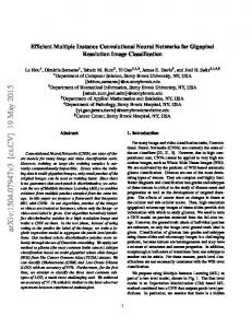
Figure 1. Illustration of the first five layers of an MSDNet with three scales. The horizontal direction corresponds to the layer direction (depth) of the network. The vertical direction corresponds to the scale of the feature maps. Horizontal arrows indicate a regular convolution operation, whereas diagonal (vertical) arrows indicate a strided convolution operation. Classifiers only operate on feature maps at the coarsest scale.

3. Problem Setup

Batch computational budget. In the batch computational budget setting, the model needs to classify a set of examples Dtest = {x1 , . . . , xM } within a finite computational budget B > 0 that is known in advance. The learner aims to minimize the loss across all examples in Dtest within a cumulative cost bounded by B, which we denote by L(f (Dtest ), B) for some suitable loss function L(·). It can B potentially do so by spending less than M computation on classifying an “easy” example whilst spending more than B M computation on classifying a “difficult” example.

We consider two settings that impose computational constraints at prediction time.

4. Network Architecture

Anytime prediction. In the anytime prediction setting (Grubb & Bagnell, 2012), there is a finite computational budget B > 0 available for each test example. The budget is nondeterministic, and varies per test instance. It is determined by the occurrence of an event that requires the model to output a prediction immediately. We assume that the budget is drawn from some joint distribution P (x, B). In some applications P (B) may be independent of P (x) and can be estimated. For example, if the event is governed by a Poisson process, P (B) is an exponential distribution. We denote the loss of a model f (x) that has to produce a prediction for instance x within budget B by L(f (x), B). The goal of an anytime learner is to minimize the expected loss under the budget distribution: L(f ) = E [L(f (x), B)]P (x,B) ,

(1)

where L(·) denotes a suitable loss function. As is common in the empirical risk minimization framework, the expectation under P (x, B) may be estimated by an average over samples from P (x, B).

Like deeply supervised networks (Lee et al., 2015) and Inception models (Szegedy et al., 2015), our convolutional network has classifiers operating on feature maps at intermediate layers in the network. Each of these classifiers can be used to output a prediction, which allows for retrieving preliminary predictions before a test image is propagated through all the layers of the network. Such preliminary retrieval is essential in both the batch computational budget setting and the anytime prediction setting. Challenges. There are two main challenges in designing network architectures that have classifiers at various layers of the network: (1) obtaining acceptable prediction accuracies at an early stage in the network whilst training a deep architecture and (2) making predictions in such a way that the computation used to evaluate early classifiers is not wasted when later classifiers are evaluated. The first challenge arises because the accuracy of classifiers that operate on low-level features (i.e., on features obtained before several levels of down-sampling) is generally low. The second challenge arises because feature maps in later layers gener-

Multi-Scale DenseNets for Efficient Prediction

ally capture different structure than features in early layers, which makes it difficult to construct classifiers that complement each other. Our convolutional networks address these two challenges via two main architectural changes. An illustration of our architecture is shown in Figure 1. Multiple scales. The first main change is that we maintain a feature representation at multiple scales in each layer2 of the network, akin to convolutional neural fabrics (Saxena & Verbeek, 2016). The feature maps at a particular layer and scale are computed by concatenating the results of one or two convolutions: (1) the result of a regular convolution applied on the same-scale features from the previous layer (horizontal connections), and if possible (2) the result of a strided convolution applied on the finer-scale feature map from the previous layer (diagonal connections). By maintaining feature representations at various scales in each layer of the network we obtain a low-resolution feature representation that is amenable to classification after just a few convolutional layers, whilst still being able to produce high-quality features (that rely on the high-resolution feature maps) later in the network. Dense connectivity. The second change we make is that we use dense connections (Huang et al., 2017) that allow each layer to receive inputs directly from all its previous layers. As shown by Huang et al. (2017), such dense connections (1) significantly reduce redundant computations by encouraging feature reuse and (2) make learning easy by eliminating the gradient vanishing problem in a way similar to residual networks (He et al., 2016). Moreover, the use of dense connections is instrumental in addressing the second challenge identified above: dense connections differ from traditional network architectures in that they add additional features at each layer whilst maintaining all features that were computed prior. Parameter efficiency. Perhaps somewhat counterintuitively, our architectural changes improve the parameter efficiency significantly. In particular, a version of our network with less than 1 million parameters is able get lower than 7.0% test error on CIFAR-10 dataset, which suggests our architecture is on par with or better than existing architectures in terms of the accuracy-model size trade-off (for instance, Saxena & Verbeek (2016) reported a 7.43% test error on the same dataset using a model with >20 million parameters). We present the details of our MSDNet below. First layer. The first layer (` = 1) is unique as it includes vertical connections in Figure 1. Its main purpose is to “seed” representations on all S scales. One could view its vertical layout as a miniature “S-layers” convolutional network (S=3 in Figure 1). Let us denote the output feature (s) maps at layer ` and scale s as x` and the original input 2

Here, we use the term “layer” to refer to a column in Figure 1.

image as x10 . Feature maps at coarser scales are obtained via down-sampling; i.e., the output of the first layer at the s-th scale is given by: ( (1) h0 (x0 ) if s = 1, (s) x1 = (s−1) ˜ h0 (x1 ) if s > 1. ˜ 0 (·) denote a regular convolutional Herein, h0 (·) and h transformation and a strided convolutional transformation, respectively. The n output of the o first layer is a collection of (1) (S) feature maps x1 , . . . , x1 , one for each scale. Subsequent layers. Following the dense connectivity pattern proposed by Huang et al. (2017), the output feature (s) maps x` produced at subsequent layers, ` > 1, and scales, s, are a concatenation of transformed feature maps from all previous feature maps of scale s and s − 1 (if s > 1). Formally, the `-th outputs a set of features n layer of our network o (1) (S) at S scales x` , . . . , x` with: h i  (s) (s)  h x , . . . , x if s = 1,  ` 1 `−1    (s)  h i  x` = (s) (s)  h x , . . . , x ,  ` 1 `−1   h i  s > 1.   ˜ ` x(s−1) , . . . , x(s−1) h 1 `−1 Herein, [. . . ] denotes the concatenation operator, h` (·) a ˜ ` (·) a strided conregular convolution transformation, and h volutional transformation. Note that the outputs of h` and ˜ ` have the same map size; their outputs are concatenated h along the channel dimension. In Figure 1, we did not draw connections across more than one layer explicitly: these connections are implicit through recursive concatenations. Classifiers. The classifiers in MSDNets also follow the dense connectivity pattern within the coarsest scale, S, at layer ` uses all the features i h i.e., the classifier (S) (S) x1 , . . . , x` . Each classifier consists of two convolutional layers, followed by one average pooling layer and one linear layer. In practice we only attach classifiers to some of the intermediate layers, and we let fk (·) denote the k th classifier. During testing in the anytime setting we propagate the input through the network until the budget is exhausted and output the most recent prediction. In the batch budget setting at testing time, an example traverses the network and exits after classifier fk if its prediction confidence (we use the maximum value of the softmax probability) exceeds a pre-determined threshold θk . Before training we compute the cost, Ck , required to process the network up to the k th classifier. We denote by 0 < q ≤ 1 a fixed exit probability that a sample that reaches a classifier will obtain a classification with sufficient confidence to exit. If q is constant across all layers we can compute the probability that a sample exits at classifier k as: qk = z(1 − q)k−1 q,

(2)

Multi-Scale DenseNets for Efficient Prediction

where z is a normalizing constant (as there are only finitely number of layers). This provides a natural way to determine the required depth of the network: as qk is exponentially decreasing, one can set the final layer to be the first layer with qk < , for some small  > 0. At test time, we need to ensure that the overall cost of classifying all samples in Dtest does not exceed our budget B, which gives rise to the constraint: X |Dtest | qk Ck ≤ B. (3) k

We can solve (3) for q and assign the thresholds θk on a hold-out set such that approximately a fraction of qk validation samples exit at the k th classifier. Loss functions. During training we use the logistic loss functions L(fk ) for each classifier and minimize the weighted cumulative loss: X 1 X wk L(fk ), (4) (x,y)∈D k |D| where D denotes the training set and wk ≥ 0 a weight of the classifier k. We can use these weights to incorporate our prior knowledge about the budget B. In the batch computational budget setting, the budget B is known before test time, which allows for the design of proper weights to adapt for the given budget. In the anytime setting, the budget B is sampled from some distribution P (x, B). When the marginal distribution P (B) is known, we can adapt the weights wk accordingly. Empirically, we find that assigning equal weights to all the loss functions, i.e., wk = 1 for all k, works reasonably well, also. Network reduction and lazy evaluation. There are three straightforward ways to further reduce the computational requirements of MSDNets. First, it is inefficient to maintain all the finer scales until the end of the network. One simple strategy to reduce the network is splitting the network into S blocks along the depth dimension, and only keep the coarsest (S − i + 1) scales in the ith block. This reduces computational cost for both training and testing. Second, we can add a transition layer between two blocks to merge the concatenated features with 1 × 1 convolution and reduce the number of channels by half, similar to the DenseNet-BC architecture (Huang et al., 2017). Third, since the classifier is only attached to the coarsest scale, finer feature maps in that layer are not used for prediction. (1) (S) Therefore, we compute the feature set {x`+1 , . . . , x`+S } in parallel, avoiding unnecessary computations when we need to stop at the (` + S)th scale to retrieve the prediction. We call this strategy lazy evaluation. Implementation details. We use MSDNet with three scales on the CIFAR datasets. The convolutional layer functions in the first layer, h1 , denote a sequence of 3 × 3 convolutions (Conv), batch normalization (BN; Ioffe &

Szegedy (2015)), and rectified linear unit (ReLU) activa˜ 1 , down-sampling is pertion. In the computation of h formed by performing convolutions using strides that are powers of two. For subsequent feature layers, the trans˜ ` are defined following the design in formations h` and h DenseNets (Huang et al., 2017): Conv(1 × 1)-BN-ReLUConv(3 × 3)-BN-ReLU. We set the number of output channels of the three scales to 6, 12, and 24, respectively. Each classifier has two down-sampling convolutional layers with 128 dimensional 3 × 3 filters, followed by a 2 × 2 average pooling layer and a linear layer. The MSDNet used for ImageNet has four scales, respectively producing 16, 32, 64, and 64 feature maps at each layer. The original images are first transformed by a 7×7 convolution and a 3×3 max pooling (both with stride 2), before entering the first layer of MSDNets. The classifiers have the same structure as those used for the CIFAR datasets, except that the number of output channels of each convolutional layer is set to be equal to the number of its input channels.

5. Experiments We evaluate the effectiveness of our approach in image classification experiments on three benchmark datasets. Code to reproduce all results is available at https:// github.com/gaohuang/MSDNet. Datasets. We perform image classification experiments on the CIFAR-10 (C10), CIFAR-100 (C100) (Krizhevsky & Hinton, 2009), and ILSVRC 2012 (ImageNet) classification (Deng et al., 2009) datasets. The two CIFAR datasets contain 50, 000 training and 10, 000 test images of 32×32 pixels; we hold out 5, 000 training images as a validation set. The datasets comprise 10 and 100 classes, respectively. We follow He et al. (2016) and apply standard dataaugmentation techniques to the training images: images are zero-padded with 4 pixels on each side, and then randomly cropped to produce 32×32 images. Images are flipped horizontally with probability 0.5, and normalized by subtracting channel means and dividing by channel standard deviations. The ImageNet dataset comprises 1, 000 classes, with a total of 1.2 million training images and 50,000 validation images. We hold out 50,000 images from the training set in order to estimate the confidence threshold for classifiers in MSDNet. We adopt the data augmentation scheme of He et al. (2016); Huang et al. (2017) at training time; at test time, we classify a 224 × 224 center crop of images that were resized to 256×256 pixels. Training details. We train all models using the framework of Gross & Wilber (2016). On the two CIFAR datasets, all models (including all baselines) are trained using stochastic gradient descent (SGD) with mini-batch size 64. We use Nesterov momentum with a momentum weight of 0.9 without dampening, and a weight decay of 10−4 . All models are

Multi-Scale DenseNets for Efficient Prediction

trained for 300 epochs, with an initial learning rate of 0.1, which is divided by a factor 10 after 150 and 225 epochs. We apply the same optimization scheme to the ImageNet dataset, except that we increase the mini-batch size to 256, and all the models are trained for 90 epochs, with two learning rate drops, after 30 and 60 epochs respectively. 5.1. Anytime Prediction We first evaluate the performance of our models in the anytime prediction setting. Here, the model maintains a predictive distribution over classes that is progressively updated. At any time during the inference process, it can be forced to output its most up-to-date prediction. Baselines. There exist two convolutional network architectures that are suitable for anytime prediction: namely, FractalNets (Larsson et al., 2017) and deeply supervised networks Lee et al. (2015). FractalNets allow for multiple evaluation paths during inference time, which vary in cost. An Anytime setting can be induced if the paths are evaluated in order of increasing cost. Here, we use the result reported in the original paper. Deeply supervised networks introduce multiple early-exit classifiers throughout a network, trained on the features of the particular layer they are attached to. Instead of using the original model proposed in Lee et al. (2015), we use the more competitive ResNet and DenseNet3 as the base networks. We refer to these as ResNetMC and DenseNetMC , where M C stands for multiple classifiers. The ResNetMC has 62 layers, with 10 residual blocks at each spatial resolution (for three resolutions): we train early-exit classifiers on the output of the 4th and 8th residual blocks at each resolution, producing a total of 6 intermediate classifiers (plus the final classification layer). The DenseNetMC consists of 52 layers with three dense blocks and each of them has 16 layers. The six intermediate classifiers are attached to the 6th and 12th layer in each block, also with dense connections to all previous layers in that block. Both networks require about 3 × 108 FLOPs when fully evaluated. In addition, we include ensembles of CNNs of identical or varying sizes. At test time, the networks are evaluated sequentially (in ascending order of network size) to obtain predictions for the test data. These predictions are averaged over the evaluated models. We experiment with ensembles of ResNets, DenseNets and a more competitive, and unpublished, variant of DenseNets (denoted as DenseNet*), that is optimized to maximize FLOP efficiency by doubling the growth rate after each transition layer. On ImageNet, we compare MSDNet against the highly 3

In all experiments, we use the state-of-the-art DenseNet with bottleneck and channel reduction layers, which is referred to as DenseNet-BC by Huang et al. (2017).

competitive ensemble of ResNets with varying depths. The ResNets we used in the ensemble range from 10 layers to 50 layers. All the models are the same as those described by He et al. (2016), except that the ResNet-10 and ResNet26 are variants of ResNet-18 that were modified by removing/adding one residual block from/to each of the last four spatial resolutions in the network. Details of architecture. The MSDNet used in our anytimeprediction experiments has 24 layers (each layer corresponds to a column in Fig. 1), using the reduced network with transition layers as described in Section 4. The classifiers operate on the output of the 2×(i+1)th layers, with i = 1, . . . , 11. On ImageNet, we use an MSDNet with 23 multi-scale layers, and the ith classifier operates on the (4i+3)th layer (with i = 1, . . . , 5). For simplicity, the losses of all the classifiers are weighted equally during training. Results. The results of our anytime-prediction experiments on the CIFAR-10 and CIFAR-100 datasets are presented in the left and middle panel of Figure 2. The figures present the classification accuracy of our models as a function of the computational budget at test time. We make two main observations. First, we observe that MSDNet substantially outperforms ResNetsMC and DenseNetsMC , in particular in regimes in which the computational budget is limited. This result is due to the fact that, unlike residual networks, MSDNets produce low-resolution feature maps after just a few layers of computations: these low-resolution feature maps are much more discriminative for classification than the highresolution feature maps in the early layers of ResNets or DenseNets. Second, MSDNet performs strongly for all budget regimes except in the extremely low-budget regime. Here, the ensemble approaches have an advantage over MSDNets, because we evaluate the smallest models in our ensembles first. In contrast to the first classifier(s) in our model, the features learned by these models are completely optimized to give rise immediate classifications, whereas the feature representations learned by MSDNet also need to maintain more complex features that are relevant for predictions produced by later classifiers. As a result, the “effective capacity” of our initial classifier (at the same number of FLOPs) is lower than that of the smallest models in the ensembles. However, this pays off quickly with increasing test time budget. In contrast, the performance of the ensembles starts to saturate as a function of the number of FLOPs, in particular, when all models in the ensemble are shallow. The rapid saturation of ensemble methods may be reduced by including increasingly deep models, but this has the downside that (unlike MSDNets) computations of similar lowlevel features are repeated multiple times. As a result, the ensembles already perform worse than MSDNet in regimes

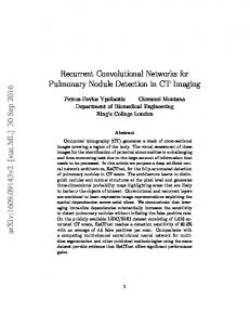
Multi-Scale DenseNets for Efficient Prediction Anytime prediction on ImageNet 76 74

+5.6%

accuracy (%)

72

MC

MC

MC

MC

70 68 66

+7.8%

64 62 60 0.0

MSDNet Ensemble of ResNets (varying depth) 0.5

1.0

1.5

budget (in FLOPs)

2.0

2.5

3.0 1e10

Figure 2. Comparison of anytime classification performance (in top-1 accuracy) on CIFAR-10, CIFAR-100 and ImageNet.

in which slightly more computational resources are available at inference time.

best classification accuracy may be achieved by performing a type of dynamic evaluation described below.

The right panel of Figure 2 shows the anytime-prediction results on ImageNet. For all budgets we evaluated, the prediction accuracy of MSDNet is significantly higher than that of the ResNet ensemble. In particular, when the budget ranges from 0.5 × 1010 to 1.0 × 1010 FLOPs, MSDNet achieves ∼ 4%−8% higher top-1 accuracy. The strong performance of MSDNet on ImageNet shows that the model is able to effectively reuse feature representations to progressively refine its predictions.

Dynamic evaluation with early-exits. We early-exit “easy” examples from a shallow classifier that is likely to produce a correct prediction for such instances with limited computation, and use the computation we saved to evaluate a deeper classifier on “hard” examples. Specifically, we associate each classifier with a confidence threshold, and let a test example exit from the first classifier at which it obtains sufficiently confident prediction, i.e., its maximum soft-max value is no less than the threshold at that classifier. The confidence threshold θk at the k th classifier is determined using the validation set, such that a proportion of qk = z(1 − q)k−1 q validation samples exit from this classifier, as defined in eq. (2).

5.2. Batch computational budget setting In the batch computational budget setting, the predictive model receives a batch of M instances and a computational budget B for classifying all instances. In this setting, the

probability density (x1e-9)

accuracy (%)

Budget distribution. To 95 Anytime learning with different distributions 8 investigate how sensitive 7 94 the performance of MSD6 93 Nets on the budget distribu5 92 tion P (B) is, we perform 4 91 experiments with three dif3 90 ferent budget distributions. 2 Uniform 89 1 The three distributions are Gaussian Exponential 88 0 illustrated in Figure 3 as 0.0 0.5 1.0 1.5 2.0 2.5 3.0 1e8 budget (in FLOPs) dotted lines: a uniform distribution, an exponential Figure 3. Classification accudistribution and a normal racies of our anytime predicdistribution. During traintion models on the CIFARing we assign weights wk 10 dataset using three differproportional to the probaent budget distributions p(B). bility that the forced exit will result in an exit after classifier fk . The results in Figure 3 show that the accuracy distributions are somewhat shifted based on the weight assignments, however, no drastic changes occur. This result provides some reassurance that the uniform weighting is probably a good choice in many real-world applications, and that we need not worry to much about errors in our estimates of p(B).

Details of architecture. The MSDNets used here for the two CIFAR datasets have depths ranging from 10 to 36 layers, using the reduced network with transition layers as deth scribed Pk inth Section 4. The k classifier is attached to the ( i=1 i) layer. The network used for ImageNet is the same as that described in the previous subsection. Baselines. On the CIFAR datasets, we compare our dynamically evaluated MSDNet with several highly competitive baselines. We include ResNets (He et al., 2016), DenseNets (Huang et al., 2017) and DenseNets* (described in Section 5.1) of varying sizes, Stochastic Depth Networks (Huang et al., 2016), Wide ResNets (Zagoruyko & Komodakis, 2016) and FractalNets (Larsson et al., 2017), with test time costs within our region of interest. For ResNets, DenseNets and DenseNet* we also introduce a cost-accuracy trade-off curve by interpolating between models of varying sizes and test-time costs Ck : Assume a given budget B falls between the costs of two such networks, such that C1 ≤ B < C2 , and in particular B = αC1 +(1−α)C2 , we randomly select a fraction α of all test instances that we classify with the network of cost C1 , and a fraction (1 − α) that we classify with the network of cost C2 . We refer to these baselines as DenseNets, ResNets and DenseNet*.

Multi-Scale DenseNets for Efficient Prediction

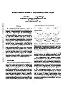
75

Batch computational learning on ImageNet ~2.2x ~2.6x ~2.3x

MC MC

MC MC

accuracy (%)

70

ResNet-50

DenseNet-121

ResNet-34 ResNet-26

ResNet-18

65

ResNet-10

MSDNet with early-exits Early-exit ensemble of ResNets ResNets (He et al., 2015) DenseNets (Huang et al., 2016) GoogLeNet (Szegedy et al., 2015) AlexNet (Krizhevsky et al., 2012)

60

0.0

0.2

0.4

0.6

average budget (in FLOPs)

0.8

1.0 1e10

Figure 4. Top-1 classification accuracy as a function of average computational cost budget on CIFAR-10, CIFAR-100 and ImageNet.

We apply the same thresholding approach, as described earlier for MSDNet, to the ResNetMC and DenseNetMC models used in Section 5.1, and perform dynamic evaluation on them. We denote these baselines as ResNetMC / DenseNetMC with early-exits. We do not experiment with deeper models as they are unlikely to be more competitive than other baselines. Our final baseline is obtained by applying the dynamic evaluation strategy to an ensemble of independently trained networks with increasing depth (we use the most competitive DenseNet* architecture). If a test input obtains an insufficiently confident prediction at a shallower network, it will be further evaluated by a deeper one, until its prediction is confident enough or it reaches the deepest model. We assign the confidence thresholds as described for MSDNet. It is worth noting that for each test input this baseline re-uses computation by ensembling the predictions of all evaluated networks. We refer to this baseline as Dynamic Ensemble of DenseNets*. On ImageNet, we compare MSDNet with five (interpolated) ResNets models described in Section 5.1, the 121layer DenseNet (Huang et al., 2017), AlexNet (Krizhevsky et al., 2012) and GoogleLeNet (Szegedy et al., 2015). In addition, we also compare with an ensemble of the five ResNets with dynamic evaluation. Results. The results of our experiments with the batch computational budget setting on the CIFAR-10 and CIFAR-100 datasets are shown in the left and middle panel of Figure 4. We trained multiple MSDNets with different depths, each of which meets a certain range of computational budget with varying exit probability q. For any given budget, the best model (shown by darker curves in the figures) is chosen based on the performance on the validation set. We observe that MSDNets consistently outperform all the baselines in terms of accuracy under the same budget. Notably, on both datasets MSDNet yields similar performance as a 110-layer ResNet using only 1/10 of the computational budget. It is also ∼ 5 times more ef-

ficient than DenseNets, Stochastic Depth Networks, Wide ResNets, and FractalNets in terms of FLOPs. The results of ResNet and DenseNet with multiple classification layers are underwhelming, which can probably be explained by the fact that earlier features in traditional convolution networks are not reliable for immediate classification. The dynamically evaluated DenseNets* ensemble (shown by the solid green curve in Figure 4) performs quite competitively on CIFAR-10, suggesting that our early-exit strategy can be potentially applied to an ensemble of convolutional networks of varying sizes. On CIFAR-100 and ImageNet, however, the ensemble only performs on par with its single-model counterpart, potentially because of a lack of consistency in the predictions of the independently trained models. In contrast, MSDNet benefits from the joint training process, leading it to consistently outperform all the baselines on both datasets. The results of MSDNet on ImageNet under the batch computational budget setting are shown in the right panel of Figure 4. The results in the figure reveal a clear trend: MSDNets with dynamic evaluation yield substantially more accurate predictions than ResNets and DenseNets with the same amount of computation. For example, given an average budget of 0.5 × 1010 FLOPs, MSDNet is able to reach ∼76% top-1 accuracy, which is ∼5% higher than that achieved by ResNets with the same number of FLOPs. Compared to the computationally more efficient DenseNets, MSDNet uses 1.6× fewer FLOPs to achieve the same classification accuracy. To illustrate the ability of our approach to reduce the computational requirements for classifying “easy” examples, we show twelve randomly sampled test images from two ImageNet classes in Figure 5. The top row shows “easy” examples, that were correctly classified and exited after the first classifier. The bottom row shows “hard” examples that would have been incorrectly classified by the first classifier but were classified correctly and exited by the final classifier. The figure suggests that early classifiers are used to

“hard” “hard”

“easy” “easy”

Multi-Scale DenseNets for Efficient Prediction

Jackel, Lawrence D, Monfort, Mathew, Muller, Urs, Zhang, Jiakai, et al. End to end learning for self-driving cars. arXiv preprint arXiv:1604.07316, 2016. Bolukbasi, Tolga, Wang, Joseph, Dekel, Ofer, and Saligrama, Venkatesh. Adaptive neural networks for fast test-time prediction. arXiv preprint arXiv:1702.07811, 2017.

Figure 5. Random example images from the ImageNet classes Red wine and Volcano. Top row: images exited from the first classification layer of a MSDNet with correct prediction; Bottom row: images failed to be correctly classified at the first classifier but were correctly predicted and exited at the last layer.

Bucilua, Cristian, Caruana, Rich, and Niculescu-Mizil, Alexandru. Model compression. In ACM SIGKDD, pp. 535–541. ACM, 2006.

rapidly classify prototypical examples of a class, whereas the last classifier is used to recognize non-typical images.

Chen, Wenlin, Wilson, James T, Tyree, Stephen, Weinberger, Kilian Q, and Chen, Yixin. Compressing neural networks with the hashing trick. In ICML, pp. 2285– 2294, 2015.

6. Conclusion We presented a study on training convolutional networks that are optimized to operate in settings with computational budgets at test time. In particular, we focus on two different computational budget settings, namely, testing under batch computational budgets and anytime prediction. Both settings require individual test samples to take varying amounts of computation time in order to obtain competitive results. We introduce a new convolutional architecture, which incorporates two changes: (1) maintaining multi-scale feature maps in early layers of the convolutional network and (2) using a feature-map concatenation approach that facilitates feature re-use in subsequent layers. The two changes allow us to attach intermediate classifiers throughout the network architecture and avoid wasted computation by re-using feature maps across classifiers. The results of our experiments demonstrate the effectiveness of these changes in settings with computational constraints. In future work, we plan to investigate the effect of these architecture changes in experiments on tasks other than image classification, e.g., image segmentation (Long et al., 2015). We also intend to explore approaches that combine MSDNets, for instance, with model compression (Chen et al., 2015; Han et al., 2015) to further improve computational efficiency.

Acknowledgements The authors are supported in part by the III-1618134, III1526012, IIS-1149882 grants from the National Science Foundation, and the Bill and Melinda Gates Foundation. We also thank Geoff Pleiss, Yu Sun and Wenlin Wang for helpful and interesting discussions.

References Bojarski, Mariusz, Del Testa, Davide, Dworakowski, Daniel, Firner, Bernhard, Flepp, Beat, Goyal, Prasoon,

Chen, Wenlin, Wilson, James, Tyree, Stephen, Weinberger, Kilian Q, and Chen, Yixin. Compressing convolutional neural networks in the frequency domain. In ACM SIGKDD, pp. 1475–1484, 2016. Deng, Jia, Dong, Wei, Socher, Richard, Li, Li-Jia, Li, Kai, and Fei-Fei, Li. Imagenet: A large-scale hierarchical image database. In CVPR, pp. 248–255, 2009. Figurnov, Michael, Collins, Maxwell D, Zhu, Yukun, Zhang, Li, Huang, Jonathan, Vetrov, Dmitry, and Salakhutdinov, Ruslan. Spatially adaptive computation time for residual networks. arXiv preprint arXiv:1612.02297, 2016. Gong, Yunchao, Liu, Liu, Yang, Ming, and Bourdev, Lubomir. Compressing deep convolutional networks using vector quantization. arXiv preprint arXiv:1412.6115, 2014. Graves, Alex. Adaptive computation time for recurrent neural networks. arXiv preprint arXiv:1603.08983, 2016. Gross, Sam and Wilber, Michael. Training and investigating residual nets. 2016. URL http://torch.ch/ blog/2016/02/04/resnets.html. Grubb, Alexander and Bagnell, Drew. Speedboost: Anytime prediction with uniform near-optimality. In AISTATS, volume 15, pp. 458–466, 2012. Han, Song, Mao, Huizi, and Dally, William J. Deep compression: Compressing deep neural network with pruning, trained quantization and huffman coding. CoRR, abs/1510.00149, 2015. Han, Song, Mao, Huizi, and Dally, William J. Deep compression: Compressing deep neural networks with pruning, trained quantization and huffman coding. In ICLR, 2016.

Multi-Scale DenseNets for Efficient Prediction

Hassibi, Babak, Stork, David G, and Wolff, Gregory J. Optimal brain surgeon and general network pruning. In IJCNN, pp. 293–299, 1993.

Lin, Tsung-Yi, Maire, Michael, Belongie, Serge, Hays, James, Perona, Pietro, Ramanan, Deva, Doll´ar, Piotr, and Zitnick, C Lawrence. Microsoft coco: Common objects in context. In ECCV, pp. 740–755. Springer, 2014.

He, Kaiming, Zhang, Xiangyu, Ren, Shaoqing, and Sun, Jian. Delving deep into rectifiers: Surpassing humanlevel performance on imagenet classification. In ICCV, pp. 1026–1034, 2015.

Long, Jonathan, Shelhamer, Evan, and Darrell, Trevor. Fully convolutional networks for semantic segmentation. In CVPR, pp. 3431–3440, 2015.

He, Kaiming, Zhang, Xiangyu, Ren, Shaoqing, and Sun, Jian. Deep residual learning for image recognition. In CVPR, pp. 770–778, 2016.

Nan, Feng, Wang, Joseph, and Saligrama, Venkatesh. Feature-budgeted random forest. In ICML, pp. 1983– 1991, 2015.

Hinton, Geoffrey, Vinyals, Oriol, and Dean, Jeff. Distilling the knowledge in a neural network. In NIPS Deep Learning Workshop, 2014.

Rastegari, Mohammad, Ordonez, Vicente, Redmon, Joseph, and Farhadi, Ali. Xnor-net: Imagenet classification using binary convolutional neural networks. In ECCV, pp. 525–542. Springer, 2016.

Huang, Gao, Sun, Yu, Liu, Zhuang, Sedra, Daniel, and Weinberger, Kilian Q. Deep networks with stochastic depth. In ECCV, pp. 646–661. Springer, 2016. Huang, Gao, Liu, Zhuang, Weinberger, Kilian Q, and van der Maaten, Laurens. Densely connected convolutional networks. In CVPR, 2017. Hubara, Itay, Courbariaux, Matthieu, Soudry, Daniel, ElYaniv, Ran, and Bengio, Yoshua. Binarized neural networks. In NIPS, pp. 4107–4115, 2016. Ioffe, Sergey and Szegedy, Christian. Batch normalization: Accelerating deep network training by reducing internal covariate shift. In ICML, pp. 770–778, 2015. Karayev, Sergey, Fritz, Mario, and Darrell, Trevor. Anytime recognition of objects and scenes. In CVPR, pp. 572–579, 2014. Krizhevsky, Alex and Hinton, Geoffrey. Learning multiple layers of features from tiny images. Tech Report, 2009. Krizhevsky, Alex, Sutskever, Ilya, and Hinton, Geoffrey E. Imagenet classification with deep convolutional neural networks. In NIPS, pp. 1097–1105, 2012. Larsson, Gustav, Maire, Michael, and Shakhnarovich, Gregory. Fractalnet: Ultra-deep neural networks without residuals. In ICLR, 2017. LeCun, Yann, Denker, John S, Solla, Sara A, Howard, Richard E, and Jackel, Lawrence D. Optimal brain damage. In NIPS, volume 2, pp. 598–605, 1989. Lee, Chen-Yu, Xie, Saining, Gallagher, Patrick W, Zhang, Zhengyou, and Tu, Zhuowen. Deeply-supervised nets. In AISTATS, volume 2, pp. 5, 2015. Li, Hao, Kadav, Asim, Durdanovic, Igor, Samet, Hanan, and Graf, Hans Peter. Pruning filters for efficient convnets. In ICLR, 2017.

Russakovsky, Olga, Deng, Jia, Su, Hao, Krause, Jonathan, Satheesh, Sanjeev, Ma, Sean, Huang, Zhiheng, Karpathy, Andrej, Khosla, Aditya, Bernstein, Michael, et al. Imagenet large scale visual recognition challenge. International Journal of Computer Vision, 115(3):211–252, 2015. Rusu, Andrei A, Rabinowitz, Neil C, Desjardins, Guillaume, Soyer, Hubert, Kirkpatrick, James, Kavukcuoglu, Koray, Pascanu, Razvan, and Hadsell, Raia. Progressive neural networks. arXiv preprint arXiv:1606.04671, 2016. Saxena, Shreyas and Verbeek, Jakob. Convolutional neural fabrics. In NIPS, pp. 4053–4061, 2016. Szegedy, Christian, Liu, Wei, Jia, Yangqing, Sermanet, Pierre, Reed, Scott, Anguelov, Dragomir, Erhan, Dumitru, Vanhoucke, Vincent, and Rabinovich, Andrew. Going deeper with convolutions. In CVPR, pp. 1–9, 2015. Trapeznikov, Kirill and Saligrama, Venkatesh. Supervised sequential classification under budget constraints. In AISTATS, pp. 581–589, 2013. Viola, Paul and Jones, Michael. Robust real-time object detection. International Journal of Computer Vision, 4 (34–47), 2001. Wan, Ji, Wang, Dayong, Hoi, Steven Chu Hong, Wu, Pengcheng, Zhu, Jianke, Zhang, Yongdong, and Li, Jintao. Deep learning for content-based image retrieval: A comprehensive study. In ACM Multimedia, pp. 157–166, 2014. Wang, Joseph, Trapeznikov, Kirill, and Saligrama, Venkatesh. Efficient learning by directed acyclic graph for resource constrained prediction. In NIPS, pp. 2152– 2160. 2015.

Multi-Scale DenseNets for Efficient Prediction

Xu, Zhixiang, Chapelle, Olivier, and Weinberger, Kilian Q. The greedy miser: Learning under test-time budgets. In ICML, pp. 1175–1182, 2012. Xu, Zhixiang, Kusner, Matt, Chen, Minmin, and Weinberger, Kilian Q. Cost-sensitive tree of classifiers. In ICML, volume 28, pp. 133–141, 2013. Zagoruyko, Sergey and Komodakis, Nikos. Wide residual networks. In BMVC, 2016.