Multiple Instance Feature for Robust Part-based Object Detection Zhe Lin University of Maryland College Park, MD 20742
Gang Hua Microsoft Live Labs Research Redmond, WA 98052
Larry S. Davis University of Maryland College Park, MD 20742
[email protected]
[email protected]
[email protected]
Abstract Feature misalignment in object detection refers to the phenomenon that features which fire up in some positive detection windows do not fire up in other positive detection windows. Most often it is caused by pose variation and local part deformation. Previous work either totally ignores this issue, or naively performs a local exhaustive search to better position each feature. We propose a learning framework to mitigate this problem, where a boosting algorithm is performed to seed the position of the object part, and a multiple instance boosting algorithm further pursues an aggregated feature for this part, namely multiple instance feature. Unlike most previous boosting based object detectors, where each feature value produces a single classification result, the value of the proposed multiple instance feature is the Noisy-OR integration of a bag of classification results. Our approach is applied to the task of human detection and is tested on two popular benchmarks. The proposed approach brings significant improvement in performance, i.e., smaller number of features used in the cascade and better detection accuracy.12
1. Introduction Pose articulation and local part deformation are among the most difficult challenges which confront robust object detection. For scanning-window-based object detectors, they produce one common issue which we call feature misalignment. It refers to the phenomenon that features which fire up in some positive detection windows do not fire up in other positive detection windows. Holistic methods [1,8,15,19,25] that concatenate local visual descriptors in a fixed order, such as HOGs [1], are inevitably cursed by this phenomenon. Part-based approaches such as [7, 11, 22] handle misalignment by training part classifiers and assembling their responses. 1 The majority of this work is carried out when Zhe Lin is an intern at Microsoft Live Labs Research. 2 We illustrate and demonstrate our approach mainly in the context of human detection while the general approach we propose can be directly applied to many other object categories such as bikes, cars, animals, etc.
(a) Global or Holistic
(b) Local, Part-based
Figure 1. Multiple instances. (a) An example of global (holistic) instances (9 instances from uniform neighborhood); (b) An example of local (part-based) instances for a two-part object (only 12 are shown among 9 × 9 instances). It is obvious that part-based multiple instances better capture articulation of a deformable object since each part can have independent placement.
Even though they can handle part misalignment somehow, training a classifier for every part might be computationally expensive. Intuitively, adopting a partbased representation in the holistic method, if appropriately modeled, may largely alleviate the feature misalignment issue. Previous work [2, 4, 6, 18] has approached this problem by allowing object parts to scale and/or shift spatially for better feature alignment, and leveraging machine learning algorithms to determine the optimal configuration of the visual parts. However, most of these approaches [4,6,18] manually picked the object parts to learn the configuration. There is no guarantee that the manual part selection would be optimal for detection. On the other hand, some boosting-based approaches [5, 16, 19, 23, 25] implicitly select visual parts, but they do not take feature misalignment into consideration. Meanwhile, multiple instance learning [14, 21] has been demonstrated to effectively handle object misalignment at the holistic level (i.e., the whole detection window). A natural question to ask is: can we extend the idea of multiple instance learning to handle the problem of feature misalignment? The answer is indeed quite straightforward by allowing multiple instances at the part levels. Figure 1 illustrates the difference between global [14, 21] and local part-based multiple instance schemes.
Hence, we introduce a framework for learning partbased object detectors which are robust to feature misalignment, and thus are robust to pose variation and local part deformation. The main idea is the introduction of a more powerful feature, or equivalently weak learner, into the Boosting framework for object detection. The new feature, called a multiple instance feature, is the Noisy-OR aggregation of the classification results of a bag of local visual descriptors. Essentially, each bag of local visual descriptors is considered as one local part of the targeted object. To efficiently utilize multiple instance features, in contrast to Dollar et al .’s work [2], which runs multiple instance learning on a randomly selected set of parts, we propose a novel seed-and-grow scheme. In essence, at each feature selection step of boosting, we first select an optimal ordinary feature, e.g., a decision stump or a decision tree. Then based on the position of the ordinary feature, we grow out to define the local part (i.e., a bag of descriptors). A multiple instance boosting algorithm [21] is further performed to obtain the optimal multiple instance feature. Our learning process is very efficient because of the proposed seed-and-grow approach. Additionally, we learn from multiple instances of both negative and positive examples and thus learning is done through very tight and fair competition between positive and negative bags. An overview of our training and testing algorithms is shown in Figure 3. Our main contributions are three-fold: • A novel boosting-based learning framework to automatically align features for object detection. • Multiple instance features for modeling part misalignment/deformations. • A seed-and-grow scheme to efficiently construct the multiple instance feature. The approach is applied to the task of human detection (see a survey [13]) and classification results are obtained on commonly used pedestrian benchmarks.
2. Multiple Instance Features 2.1. Aggregating Multiple Instances A multiple instance feature basically refers to an aggregation function of multiple instances. More specifically, given a classifier C, it is the aggregated output, y, of a function, f , of classification scores, {yj }j=1...J , of multiple instances, {xj }j=1...J : y = f (y1 , y2 , ...yJ ) = f (C(x1 ), C(x2 ), ...C(xJ )). (1) Suppose we have a set of labeled bags {xi , ti }i=1...n where label ti ∈ {0, 1}. A bag xi consists of a set of
instances: xij , j = 1...Ni . The number of bags is n, and Pn the number of instances is N = i=1 Ni . Given a realvalued (real-valued output) classifier C, the score yij of an instance xij can be computed as: yij = C(xij ). The probability of an instance xij being positive is modeled by the standard logistic function [21] as: pij = p+ ij = 1 . 1+exp(−yij ) In [9], a multiple instance learning problem is formulated as the maximization of diverse density which is a measure of intersection of the positive bags minus the union of negative bags. The diverse density is probabilistically modeled using a Noisy-OR model for handling multiple instance learning problems. Under this model, the Q probability of a bag being positive is given Ni by pi = 1− j=1 (1−pij ). We modify this by taking the geometric mean to avoid numerical issues when Ni is Q Ni 1/Ni . (1 − pij )) large, so instead, we use pi = 1 − ( j=1 Intuitively, the model requires that at least one instance in each positive bag has a high probability, while all instances in each negative bag have low probabilities. In terms of scores, the multiple instance aggregated score yi is computed from instance scores yij as:
yi = log
Y
(1 + eyij )
k
!1/Ni
− 1,
(2)
which can be easily derived from the relation between 1 pi and yi , i.e. pi = 1+exp(−y . We refer to the above ij ) aggregated score computed from Equation 2 as multiple instance feature.
2.2. Learning Multiple Instance Features Learning multiple instance features involves estimation of the function f and instance classifier C. Assuming that the aggregation function f is given as the Noisy-OR integration, we can learn the instance classifier C via multiple instance boosting (MILBoost), which was originally introduced in [21], as an application of the diverse density to rare event detection problems to handle misalignment of examples in training images. In MILBoost, each training example is represented as multiple instances residing in a bag, and the bag and instance weights are derived under the Anyboost framework [10] which views boosting as gradient descent. Given an adaboost classifier C = {λt , ht (·)}t=1...T , the score yij of an instance xij is computed as a weighted sum of scores from all weak classifiers ht (x): yij = C(xij ) =
X
λt ht (xij ),
t
where ht (x) ∈ {−1, +1} and the weight λt > 0.
(3)
The overall likelihood assigned to a set of labeled training bags is Y 1−t pi ti (1 − pi ) i . (4) L(C) = i
Hence, the learning task is to design a boosted classifier C so that the likelihood L(C) is maximized. This is equivalent to maximize the log-likelihood X ti log pi + (1 − ti ) log (1 − pi ). (5) log L(C) = i
According to the Anyboost framework [10], the weight of each example is given as the partial derivative of the likelihood function (which can be regarded as a negative cost function) w.r.t. a change in the instance score yij . Hence, the instance weights wij can be derived (see appendix for the detailed derivation) as: ∂ log L(C) 1 ti − p i = wij = pij , ∂yij Ni p i
(6)
where the weights for positive and negative examples − + 1 i are wij = N1i ti −p pi pij and wij = − Ni pij , respectively. Interestingly, the formula for the weight values are exactly 1/Ni -scaled versions of the ones derived in [21]. The boosting process is composed of iterative weight updates and additions of weak hypotheses. Based on [10,21], each round of boosting is conducted through the following two steps: • search for the optimal weak classifier h(x) ∈ {−1, +1} which maximizes the energy function ψ(h): X t wij h(xij ) (7) ψ(h) = ij
t and set the under the current weight distribution wij optimal weak hypothesis as ht+1 . Pt t • given the previous classifier C t (x) = τ λt h (x) and the currently chosen weak classifier ht+1 , search for the optimal step size λ∗t+1 so that L(C t (x) + λt+1 ht+1 (x)) is maximized, and set C t+1 (x) = C t (x) + λ∗t+1 ht+1 (x).
We learn multiple instance features at the part level, and adopt them as potential weak classifiers for learning boosted deformable object detectors, which is discussed in Sec. 3 in detail.
3. Part-based Object Learning Modeling deformable objects as a composition of parts is a well-studied approach to object recognition. For example, the pictorial structure model [3] represents an object as a set of visual parts placed in a deformable configuration, where the appearance of each part is modeled separately and deformation is modeled as a set of spring-like connections between parts. In object detection, most existing part-based
Figure 2. An example of part-based object model learning. The learning process consists of iterative modules of discriminative part selection and part classifier learning.
approaches [7, 11, 12, 22] manually decompose an object into semantic parts such as head-shoulder, torso, and legs. In contrast, we aim for automatically selecting discriminative parts through training on labeled examples.
3.1. Learning Framework
Suppose the object of interest to be modeled consists of L parts (L is given). Each part is assumed to be square or rectangular blocks or regions3 . The learning algorithm should automatically figure out the most discriminative combination of L parts (or regions) among the set of Np candidate visual parts: P = {P1 , ...PNp }. A part Pj is represented as a set of instances which correspond to a set of locally neighboring (possibly overlapping) local image regions.4 From each instance (an image region) of a part, a predefined feature set Fj is computed and a subset of those features are chosen to contribute to the final strong classifier. From each selected part, a fixed number of weak classifiers are learned and added to the final strong classifier. Our object model learning framework is visualized in Figure 2. It adopts an efficient seed-and-grow scheme to boost multiple instance features. The framework first selects the most discriminative part by locating a seed feature from the whole feature pool, and then training the part’s classifier using multiple instance boosting by adding features to that part (i.e. growing). The two modules are repeated to progressively select parts and learn their classifiers. Note that the learning process focuses on a single part (region) at a time, i.e., multiple instances are only considered for the currently active part. After a part is learned, all features belong to that part are removed from the current feature pool so that it will not be selected again. The first feature (or weak classifier) for the next part is chosen from the remaining (unexplored) feature pool as in the ordinary 3 The regions can be arbitrary regions in a detection window and need not to be semantic object parts. 4 Given a potential part and a training example, a bag includes (feature) instances extracted from a set of neighboring local image regions around the part’s default location. The set of neighboring image regions can be obtained either by jittering the default part region or uniformly sampling regions in spatialscale space around the default location.
boosting approach. Then the region (or block) corresponding to that part is localized. Next, subsequent (2nd, 3rd,...) weak hypotheses of that localized part are learned using MILBoost [21] (see Sec. 2.2). In this boosting framework, part selection and weak classifier training are simultaneously performed. Part selection provides a weak learner pool for the current boosting round. The final strong classifiers are constructed by boosting multiple instance features from selected parts. The multiple instance features are directly used as additive weak hypotheses to construct the final strong classifier (see Figure 3).
3.2. Weak Classifiers for Multiple Instance Features
As mentioned before, for constructing a cascade classifier, the training algorithm needs to repeatedly add weak learners ht (x) to the classifier C. Each weak learner ht (x) is chosen based on the criterion P t of maximizing ψ(h) = ij wij ht (xij ). Instead of binary stumps [20], we use more informative domainpartitioning weak classifiers as in [17], where each weak hypothesis makes its prediction based on a partitioning of a feature’s domain X into disjoint regions X1 , ...XK . Suppose we partition the domain of h(x) into K bins and assign binary values ck = {+1, −1} to each bin k = 1, 2..K, i.e., ck = h(x) for x ∈ Xk . The goal is to find the optimal weak hypothesis h∗ (x) (consisting of the K − 1 partition thresholds and the binary values {ck }k=1,2...K ) such that ψ(h) is maximized. Finding partition thresholds is equivalent to learning a binary decision tree with blog2 Kc levels, e.g. for K = 8, we learn a three-level decision tree classifier. For each feature, a greedy optimization process is applied to adjust the partition thresholds (by an iterative binary splitting algorithm) and optimal score values ck for the partitioned intervals are determined so that ψ(h) can be minimized for that feature. For each k and for b ∈ {−1, +1}, let X wij . (8) Wbk = ij:xij ∈Xk ∧tij =b
Then, ψ(h) in Equation 7 can be rewritten as: X X X wij h(xij ) = ck (W+k + W−k ). ψ(h) = k ij:xij ∈Xk
k
(9) This means that we only need to choose ck based on the sign of W+k + W−k , i.e., ck = sgn(W+k + W−k ). All that remains is to estimate the step size αt for the chosen weak hypothesis ht (x) = h∗ (x) so that the objective function L(C + λt ht ) is maximized. This is done by line search in some interval [0, γ] (γ = 5 and search step size as 0.01 are shown to be adequate in our experiment).
Figure 4. Visualization of an example feature selection process (better viewed in color). Red, green and blue square blocks denote 1st, 2nd and 3rd scale/resolution level features respectively. Columns from left to right indicate features selected in different stages of the learning algorithm, and the final column shows accumulated evidence.
The resulting step sizes λt from the above process are uniformly assigned to all intervals of a feature’s domain. This poses the question of how we can generalize it to confidence-rated step sizes (nonuniform step sizes λkt for different interval k). We introduce a greedy optimization to improve the step sizes as follows: • initialize step sizes λt,k = λt , k = 1, 2...K • for k=1:K – search over an interval (λt −δ, λt +δ), find maximum likelihood estimation λt,k = λ∗t,k so that L(C, λ∗t,1 , ..., λ∗t,k−1 , λt,k , ...λK t ) is maximized. • endfor • return λ∗t,1 , ..., λ∗t,K .
The overall training and testing algorithms are shown in Figure 3. We assume that both positive and negative examples consist of multiple instances and reside in bags so that a discriminative classifier can be learned via a tight competition between positive and negative examples. An example visualization of part selection is shown in Figure 4. As we can see, most discriminative parts are selected in legs, head, head-shoulder areas and more features are chosen from salient regions around human silhouette boundaries.
4. Implementation We use multi-scale, multi-resolution shared HOG feature descriptors as the feature pool of our object learning and detection algorithms. The descriptor is a multi-resolution generalized version of histograms of oriented gradients (HOGs) [1] and is formed by extracting and concatenating dense descriptor elements from multiple resolutions. A descriptor element is a 36-dimensional vector computed from a 2 × 2-cell spatial block. Descriptor elements computed at higher pyramid levels correspond to larger spatial blocks at lower resolutions. We concatenate all descriptor elements (from three different resolution levels in which
TRAINING ALGORITHM Input: ? Labeled training examples {xi , ti }i=1...N , where ti ∈ {0, 1}. ? The number of parts to learn L and a pool of candidate parts Pj , j = 1, 2..Np . Each part j corresponds to a set of bags {xij , ti }i=1...N , where each bag xij consists of instances {xijk , ti }i=1...N . Initialization: ? Initialize weights wi , i = 1...N such that wpos =
Nneg Npos +Nneg
and wneg = − N
Npos pos +Nneg
.
? Set F 1 ← F , classifier C ← φ (empty set), and example scores yi ← 0, i = 1...N , where F = F1 ∪ F2 ... ∪ FNp is the set of all features from all candidate parts. Training: For l = 1...L: ? From F l , form a weak learner h (corresponding to a feature fmn ) to maximize adaboost setting (no multiple instances are allowed), and set hl1 = h. ? Localize a part based on feature fmn and set the part index as IDX(l) = m. P Tl PT l l λlt hlt (x) = t=1 ct (x). ? Train a MILBoost classifier C l , y = C l (x) = t=1
PN
i=1
wi h(xi ) under the ordinary
? Update the overall strong classifier as: C ← C + C l .
? Use Equation 2 to compute the multiple instance features yil for all i = 1...N . ? Update example scores by boosting multiple instance features yil , i = 1...N , yi ← yi + yil . ? F l+1 = F l − Fm . (remove all features belonging to part m from the current feature pool.) ? Set the rejection threshold rth(l) of stage l as the minimum positive score: minti =1 {yi } . Output: Overall classifier C = {C l }l=1...L and the set of rejection thresholds {rth(l)}l=1...L . TESTING ALGORITHM For a test example x, set the initial score y = 0 For l = 1...L: ? Use Equation 2 to compute the multiple instance feature yl , and update the score y ← y + yl . ? if y < rth(l), reject; else continue. Decide positive if l = L and y ≥ rth(L); else negative. Detection confidence: prob =
1 . 1+exp(−y)
Figure 3. Part-based Object Learning and Testing Algorithms.
consecutive levels differ by a factor of 2) which are relevant to a detection window to form the descriptor for that window. Hence, for a typical 64 × 128 pedestrian detection window, there are total of 105 + 21 + 3 = 129 spatially overlapping blocks. The dimensionality of the descriptor is 36 × 129 = 4644.5 In the object learning algorithm implementation (see Figure 3), each training and testing example xi represents a 64 × 128 image patch, and each candidate part Pj is defined as a HOG block (one of 129 multiresolution blocks) and its feature pool Fj consists of 36 features (i.e. HOG features of a block). The overall set of features is F = F1 ∪ F2 ... ∪ FNp and the feature set of each part Pj is represented as the feature pool Fj = {fj1 ...fjd } for part j. Each part j of an example xi is modeled as a bag denoted as xij and instances of the bag is denoted as xijk . We fix the number of weak learners for a part to be a constant (Tl = T, l = 1, 2...L) in our current implementation. 5 In this section and the algorithm in Figure 3, the meanings of subscripts i, j, k are example, part and part instance, respectively, and are different from previous sections.
In practice, instead of adding a fixed number of weak classifiers for each part, we use an adaptive method by adding weak learners until the contribution of the next weak hypothesis falls below some threshold δP> 0, i.e. terminate adding weak hypothesis when ik wijk ht (xijk ) < δ (where i, j, and k denote example, part, part instance, respectively) or the step size is small λt < δ.
5. Experiments 5.1. Datasets We use the INRIA person dataset6 [1] and the MITCBCL pedestrian dataset7 [12, 15] for performance evaluation. In these datasets, training and testing samples all consist of 64 × 128 image patches. Negative samples are randomly selected from raw (person-free) images; positive samples are cropped (from annotated images) such that persons are roughly aligned in location and scale. The MIT-CBCL dataset contains 6 http://lear.inrialpes.fr/data 7 http://cbcl.mit.edu/software-datasets/ PedestrianData.html
Detection Error Tradeoff (DET) curves
−1
10
−2
10
Detection Error Tradeoff (DET) curves
inria−mil24−dim4644−nwls96 inria−mil24−dim4644−nwls192 inria−mil24−dim4644−nwls288 inria−mil24−dim4644−nwls384 inria−mil24−dim4644−nwls480 inria−mil24−dim4644−nwls576 inria−mil24−dim4644−nwls648
−1
10
Miss Rate
inria−mil18−dim4644−nwls72 inria−mil18−dim4644−nwls144 inria−mil18−dim4644−nwls216 inria−mil18−dim4644−nwls288 inria−mil18−dim4644−nwls360 inria−mil18−dim4644−nwls432 Miss Rate
Miss Rate
Detection Error Tradeoff (DET) curves
−5
−4
−3
−2
10 10 10 10 False Positives Per Window (FPPW)
−1
10
10
−6
−5
10
−4
−3
−2
10
−1
10 10 10 10 False Positives Per Window (FPPW)
10
(a) INRIA dataset(nwls per part=18) (b) INRIA dataset(nwls per part=24)
−6
10
−5
−4
−3
−2
10 10 10 10 False Positives Per Window (FPPW)
−1
10
(c) INRIA dataset(multi-line-search)
Detection Error Tradeoff (DET) curves
inria−mil18−dim4644−nwls432 inria−mil24−dim4644−nwls648 Class. on Riemannian Man. Dalal&Triggs, Ker. HoG Dalal&Triggs, Lin. HoG Zhu et al. Cascade of Rej.
mit−mil−nwls432 mit−mil−nwls648
−1
10
10
Miss Rate
Miss Rate
Detection Error Tradeoff (DET) curves
−1
−1
10
−2
−2
−6
10
inria−mil18−dim4644−nwls72 inria−mil18−dim4644−nwls144 inria−mil18−dim4644−nwls234 inria−mil24−dim4644−nwls96 inria−mil24−dim4644−nwls192 inria−mil24−dim4644−nwls336
−2
10 −2
10
−6
10
−5
−4
−3
−2
10 10 10 10 False Positives Per Window (FPPW)
−1
10
(d) INRIA dataset(comparison)
−6
10
−5
−4
−3
−2
10 10 10 10 False Positives Per Window (FPPW)
−1
10
(e) MIT-CBCL dataset(evaluation)
Figure 5. Performance evaluation results on the INRIA dataset (nwls means number of weak classifiers). (a) Evaluation of our part-based detectors (18 weak classifiers for a part) with increasing numbers (72-432) of weak classifiers. (b) Evaluation of our part-based detectors (24 weak classifiers for a part) with increasing numbers (96-576) of weak classifiers. (c) Evaluation of our (multi-line-search) part-based detector. (d) Two detectors trained using our part-based approach are compared to HOG-Ker.SVM [1], HOG-Lin.SVM [1], HOG Cascade [25], and Classification on Riemannian Manifolds [19]. The results of [1] are approximate and are obtained from the original paper, and the results of [19, 25] are obtained by running their original detectors on the test data. (e) Evaluation of the two detectors (trained on the INRIA dataset) on the MIT dataset. Table 1. Other comparison results on the INRIA dataset. Miss rates(%) (with respect to FPPW values) are compared. Results of [2, 6, 8, 14] are approximate and are obtained from their original papers for comparison purposes. FPPW 1e-6 1e-5 1e-4 1e-3
[2] N/A 15.0 4.0 1.5
[14] N/A 7.2 4.2