Neural Network Based Priority Assignment for Job Scheduler ... manufacturing, computer processing, transportation, health care, space exploration, and ...
AU J.T.9(3): 181-186 (Apr. 2006)
Neural Network Based Priority Assignment for Job Scheduler Kothalil Gopalakrishnan Anilkumar and Thitipong Tanprasert Faculty of Science and Technology, Assumption University Bangkok, Thailand
Abstract This paper describes the design and implementation of a neural network-based job priority assigner system for a job scheduling environment. Scheduling deals with the allocation of resources over time to perform a collection of tasks. Scheduling problems arise in domains as diverse as manufacturing, computer processing, transportation, health care, space exploration, and education. In the case of a neural network (NN) based scheduler, once the job attributes are properly trained for a specified schedule, it will never miss that related scheduling pattern for that particular job. An NN based scheduling procedure can successfully overcome the local minima of its error surface. This paper reports on research which established that a back propagation neural network-based priority procedure would recognize jobs from a job queue by estimating each job’s priority. Once the priorities are assigned, it is not possible to alter the priorities under any circumstances. Keywords: Backpropagation, priority, queue, deadline, resource, processing time.
Introduction
Fuzzy based scheduling allows the representation by fuzzy sets and linguistic variables and inference from vaguely formulated knowledge (Slany 1994). The main disadvantage is the tremendous computational effort that is needed to handle the complex industrial problems. Also, they need to maintain a huge fuzzy knowledge base (rules) which is a time-consuming process. Inflexibility of the artificial neural network (ANN) in job scheduling was detected by (Zweben 1994) while investigating the use of neural network in optimization problems (Interante 1997). Apart from the priority assigner design, the intention of our research was to carryout certain studies to find out a suitable feed forward NN for job scheduling environment. The analysis used the famous backpropagation algorithm (Rao 1996) for testing various NN topologies. The organization of this paper is as follows. After the introduction, the neural network selection section describes the various testing and simulations to find a suitable NN. Next, the priority assigner design section presents in detail the model of NN based priority assigner. After that, the testing section describes computer simulation of the assigner. Finally the conclusion section concludes this paper.
Scheduling refers to the act of assigning resources to tasks or assigning tasks to resources. One way to do this is to generate a timetable with explicit start times for each task in such a way that only one task at a time requests the resource. This is often called static scheduling or timetable scheduling. This is the way airliners schedule their flights. Another solution for scheduling is to assign numbers, called priorities, to the tasks and choose for execution the task with the highest priority. Scheduling decisions occur whenever there are more outstanding requests than the number of available resources. The exact priority assigned is unimportant; only the relative priority order is important because it determines which tasks are the highest priority ones. With scheduling based on priorities instead of a timetable, there is no loss of generality because if one can change priorities at any time and also have the option of introducing idle tasks, then one can emulate every timetable. There are many approaches used to find solutions to job scheduling problems. Dispatch rules have been used to solve job scheduling problems (Baker 1984). These rules lack a global view of the shop and they usually build up a large amount of bottleneck in a complex industrial situation. 181
AU J.T.9(3): 181-186 (Apr. 2006)
The training result of the selected neural network (3 35 1) using the conventional backpropagation algorithm is shown in Fig. 1. It was found that the MSE was reduced to a value of less than 10% after 45000 epochs. This means that the algorithm took long time to reach an optimal solution level.
Neural Network Selection After testing of various possible neural network topologies, we decided to select a NN with topology 3 35 1 (one input layer one hidden layer and an output layer) which is the optimal one with a learning rate of 0.4. Before implementing the decided neural network to the assigner, two features of back propagation algorithm were used to test the neural network for the best possible result. The details of the analysis carried out are given below:
B. Testing Backpropagation Algorithm with Momentum Term A simple modification of the training law results in faster training through the addition of a momentum (β) term. That is, a momentum term was added to the weight change section of the backpropagation algorithm as follows: weight_change = learning_rate * output_ error * inputdata + momentum *previous_ weight_change (1)
A. Testing Backpropagation Algorithm without Momentum Term Backpropagation algorithm is the most popular supervised training algorithm. As the name implies, an error in the output node is corrected by back propagating this error by adjusting weights through the hidden layer and back to the input layer. The process of error propagation is repeated until the mean squared error (MSE) of the output is sufficiently small. The forward pass of the algorithm computes the neuron activations and an output. The backward pass of the algorithm computes the gradient (with respect to the given data sample). The weights are then updated so that the error is minimized.
Therefore the new_weight is; new_weight = current_weight + weight_ change (2) Implementation of the Momentum Term To accumulate the current cycle weight changes in a vector, current_wt and the past cycle weight changes were stored in a vector, past_wt. The updateweights() routine was: update_weights (float alph, float beta) { int i, j, k,inputs,outputs; float weight_change; for(i =0; i < inputs; i++){ k = i*outputs; for(j=0; j < outputs; j++) {weight_change=alpha*output_errors[j]*(inpu ts+i)+beta* past_wt[k+j]; new_weight[k+j] += weight_change; current_wt[k+j] += weight_change;}}} When a new cycle began, the past-wt pointer was swapped with the current-wt pointer. That is, the contents of the current_wt became zero for the new cycle, which was implemented by update_beta() function in the scheduling program.
Fig.1. Training result of the neural network without momentum term. 182
AU J.T.9(3): 181-186 (Apr. 2006)
1. Began with a set of jobs (jobs are in a job queue). 2. Got basic attributes related to each job’s such as deadline, resource(s) and processing time. 3. Trained the scheduler with the mentioned job attributes that covers all set of possible combinations of the application environment. 4. Got the attributes of a job set from the user. 5. Trained the entered attributes with precalculated weights. 6. Displayed the job sequence based on their priorities by appending the sorted job queue and priority queue. 7. Went to step 1 for next set of jobs.
The network weight change in the absence of error and input data would be a constant multiplied by the previous weight change. The momentum term (β) was an attempt to try to keep the weight change process moving, and thereby not get network stuck in local error minima. The training result of the network (topology 3 35 1) with momentum term is shown in Fig.2.
We assumed that a job is divided into different sub sets and all jobs were available in a job queue. The size of a job set was obviously equal to the size of the job queue. Once the priority was assigned, a new job set was entered into the job queue. The input data sets of the neural network had 3 job attributes (deadline, resource and processing time). The priority assigner architecture is shown in the Fig. 3.
Fig.2. Training result of the neural network with momentum term The MSE was reduced to a value of less than 10% after 14800 epochs. That is, the algorithm provided faster results. After testing with various values, the momentum was fixed at 0.018 for getting optimum results. Details of the NN parameters after the analysis were:
A. Job Queue We assumed that a job queue J has n possible jobs based on their arrival are shown below:
Learning rate (∝) = 0.4 Maximum error tolerance = 0.009 Momentum term (β) = 0.018 Neural network topology = 3 35 1
Ji
From the experimental analysis, it was found that the momentum term along with weight changing procedure in backpropagation algorithm improved the training speed and the training result as well.
= :
J1 J2 Jn
Where i = 1, 2,….., n.
Priority Assigner Design Using the Selected Neural Network
B. Priority Queue The estimated job priority was available in a priority queue P, which is shown below:
The analyzed three layer feed forward backpropagation NN was now ready to be implemented. The procedure used in the implementation of the priority assigner is given below:
Priority, Pj = 183
P1 P2 :
AU J.T.9(3): 181-186 (Apr. 2006)
In our research, it was assumed that the deadline, resource, and processing time of each job are known in advance and that the system had a user interface section which accepts user input for each job. The neural network with job queue, job attributes, and priority queue is shown in Fig. 4.
Pn Where j = 1, 2, … , n
Priority Extraction: In this experiment, apart from the ‘black box’ concept of the NN, we used a knowledge concept to fix the initial data set. The knowledge is described in the form rule is given as: If deadline is very near AND resource is very high AND processing_time is very low, then priority is very high. From the above rule, the following proportionalities were concluded; a. priority α deadline b. priority α resource c. priority α ( 1/processing_time)
Fig. 3. Priority assigner architecture.
Based on the given proportionalities, (approximate) derivation for the priority was; priority ≈ (deadline * resource)/processing_time (3) Therefore, the initial data set of the NN was more or less similar to the Equation (3). This way, we eliminated the occurrence of ‘over fitting’ of data during the training process. The estimated priority value wasnot allowed to exceed more than 0.99. If it did, the NN always gave a default result of 0.99. The range of input data values defined for NN training was 0.10 to 0.90.
Testing and Analysis The assigner recognized each job based on their priority order, by appending the sorted job queue along with the priority queue. There are two simulation results are depicted here; Table 1 shows simulation result with first set of *unseen input for 8 jobs and Fig.5 shows the job order based on their priorities (which are indicated in Table 1).
Fig. 4. Neural network with job queue attributes and priority queue. 184
AU J.T.9(3): 181-186 (Apr. 2006)
the priority predictor is more than 98% (by correlation) accurate with any input which were in the range 0.10 to 0.90.
Table 1 JOB Name JOB1 JOB2 JOB3 JOB4 JOB5 JOB6 JOB7 JOB8
Priority 0.384 0.792 0.537 0.364 0.685 0.925 0.550 0.909
Table 3 Deadline Resource Processing Priority time 0.35 0.78 0.70 0.390 0.67 0.90 0.80 0.750 0.25 0.54 0.30 0.450 0.40 0.65 0.75 0.346 0.50 0.60 0.48 0.625 0.90 0.80 0.75 0.960 0.45 0.87 0.69 0.567 0.89 0.67 0.64 0.931
Fig.5. Job order given by the simulator based on the table 1.
Table 4
Similarly, Table 2 shows simulation result with second set of unseen input for 8 jobs and Fig.6 shows corresponding job order.
Deadline Resource Processing Priority time 0.35 0.78 0.70 0.384 0.67 0.90 0.80 0.792 0.25 0.54 0.30 0.537 0.40 0.65 0.75 0.364 0.50 0.60 0.48 0.685 0.90 0.80 0.75 0.925 0.45 0.87 0.69 0.550 0.89 0.67 0.64 0.909
Table 2 JOB Name JOB1 JOB2 JOB3 JOB4 JOB5 JOB6 JOB7 JOB8
Priority 0.663 0.618 0.796 0.626 0.381 0.951 0.418 0.294
Table 5 Deadline Resource Processing Priority time 0.43 0.47 0.32 0.632 0.57 0.67 0.69 0.553 0.39 0.40 0.20 0.780 0.80 0.70 0.91 0.615 0.37 0.47 0.48 0.362 0.49 0.79 0.39 0.992 0.57 0.29 0.40 0.413 0.21 0.31 0.24 0.271
Fig.6. Job order given by the simulator based on the table 2. Table 3 and Table 5 show the priority results after applying the equation (3) on set of unseen input set for 8 jobs. Similarly, Table 4 and Table 6 show the result from the simulator with the same set of unseen inputs (as given in table 3 and table 5). By comparing the priorities from the first (tables 3 and 4) and second (tables 5 and 6) pairs, it was found that
* The input combinations which are not included in the initial training set are considered as ‘unseen’. 185
AU J.T.9(3): 181-186 (Apr. 2006)
Through this priority assigner simulator, it is noticed that the trained NN will always provide proper responses to any unseen situations. This ability of the NN is considered as one of the key strengths of the neural network based designs. Finally, the overall conclusion is that backpropagation networks are suitable for any type of prediction problems.
Table 6 Deadline Resource Processing Priority time 0.43
0.47
0.32
0.663
0.57
0.67
0.69
0.618
0.39
0.40
0.20
0.796
0.80
0.70
0.91
0.626
0.37
0.47
0.48
0.381
0.49
0.79
0.39
0.951
0.57
0.29
0.40
0.418
0.21
0.31
0.24
0.294
References Baker, K.R. 1984. Introduction to Sequencing and Scheduling. Wiley, New York, NY, USA.. Interante, L.D. 1997. Artificial Intelligence and Manufacturing: A Research Planning Report. AAAI/SIGMAN, Albuquerque, NM, USA. Rao, B.; and Rao, H.V. 1996. Neural Networks & Fuzzy logic, BPB Publ., Delhi, India. Slany, W. 1994. Scheduling as a fuzzy multiple criteria optimization problem. CDTechnical Report 94/62, Technical University of Vienna, Vienna, Austria. Zweben, M.; and Fox 1994. Intelligent Scheduling. Morgan Kaufman. New York, NY, USA.
Conclusion In this paper, it was proved that the NN based assign procedure can predict successfully any problem sequence. Trained NN represents equivalent form of dispatching rules. Hence the greatest advantage of the NN is that, it will provide ‘rule less’ solution environment for an application. The rules are always rigid but the neural network based designs are never rigid.
186