Three of the popular approaches for feedback control of a two-dimensional wake are direct feedback ...... 1Gillies, E. A.., “Low-dimensional Control of the Circular Cylinder Wake”, Journal of Fluid Mechanics, Vol. 371 ... 182, 1993, pp. 244, 248.
AIAA 2006-6428
AIAA Guidance, Navigation, and Control Conference and Exhibit 21 - 24 August 2006, Keystone, Colorado
Neural Network Estimator for Closed-Loop Control of a Cylinder Wake Young-Sug Shin*, Kelly Cohen*†, Stefan Siegel‡, Jürgen Seidel § and Thomas McLaughlin ** Department of Aeronautics US Air Force Academy US Air Force Academy, CO 808400
Downloaded by UNIVERSITY OF CINCINNATI on December 7, 2014 | http://arc.aiaa.org | DOI: 10.2514/6.2006-6428
The effectiveness of a non-linear Artificial Neural Network Estimator (ANNE) for feedback flow control on the wake of a circular cylinder is investigated in direct numerical simulations. The research program is aimed at suppressing the von Kármán vortex street in the wake of a cylinder at a Reynolds number of 100. Various configurations of sensors, varying both number and location, were studied from just one sensor through 4 sensors. A low-dimensional Proper Orthogonal Decomposition (POD) is applied to the flow field velocity and sensor placement is based on the intensity of the resulting spatial Eigenfunctions. The numerically generated data was comprised of 138 snapshots taken over 11 cycles from the periodic regime. A Linear Stochastic Estimator (LSE) was employed to map the velocity data to the temporal coefficients of the reduced order model and results are compared with those obtained using ANNE. All sensor configurations were studied for four different cases, namely, noiseless data and three levels of increasingly degraded data by injection of random noise. For a given four sensor configuration, ANNE was compared to LSE, Quadratic Stochastic Estimation (QSE) and LSE with time delays (DSE). We show ANNE to be far more robust and accurate in comparison to all of these procedures. Nomenclature an (t) bn Cns Cd D f fa FD gk Re St Si
~ u ( x , y, t )
U ( x , y)
U∞ u (x, y, t) x, y α Ф (x, y) υ
= = = = = = = = = = = = = = = = = = = =
Time dependent coefficient, of nth mode, of the low-dimensional model Coefficients associated with the control input, of nth mode, of low-dimensional model Coefficients of the linear stochastic estimator Mean drag coefficient Cd = FD / .5 ρ U∞2 .D.1 Cylinder Diameter Vortex shedding frequency Feedback control input to the cylinder Drag Force Quadratic nonlinear function used in low-dimensional, time-depending model Reynolds number Re = U∞ D / υ Strouhal number St = f D / U∞ Sensor measurement of stream-wise velocity. “i’ is the number of the sensor Velocity field Mean flow Freestream velocity Fluctuating velocity component Spatial coordinates Skew angle of attack of the incoming flow used to trigger CFD simulation Spatial Eigenfunction or POD mode Kinematic viscosity
*
ESEP Researcher from Korea, Department of Aeronautics, US Air Force Academy, Member, AIAA Contracted Researcher, Department of Aeronautics, US Air Force Academy, Senior Member, AIAA ‡ Contracted Researcher, Department of Aeronautics, US Air Force Academy, Senior Member, AIAA § Contracted Researcher, Department of Aeronautics, US Air Force Academy, Member, AIAA ** Director of Research, Aeronautical Research Center, US Air Force Academy, Associate Member, AIAA *†
1 American Institute of Aeronautics and Astronautics This material is declared a work of the U.S. Government and is not subject to copyright protection in the United States.
Downloaded by UNIVERSITY OF CINCINNATI on December 7, 2014 | http://arc.aiaa.org | DOI: 10.2514/6.2006-6428
I.
Introduction
One of the main purposes of flow control is the improvement of aerodynamic characteristics of air vehicles and munitions enabling augmented mission performance. An important area of flow control research involves the phenomenon of vortex shedding behind bluff bodies. These bodies often serve some vital operational function. Their purpose is not to augment aerodynamic efficiency and often aerodynamic performance is sacrificed for functionality. Flow separates from large section of the bluff body’s surface. The resulting wake behind the bluff body exhibits vortex shedding, which then leads to a sharp rise in drag, noise and fluid-induced vibration1. The intensity of the undesired aerodynamic characteristics associated with wake flow may be reduced by introducing flow control mechanisms. The ability to control the wake of a bluff body could be used to reduce drag, increase mixing and heat transfer, and enhance combustion2-4. Shedding of counter-rotating vortices is observed in the wake of a two-dimensional cylinder above a critical Reynolds number (Rec ~ 47, nondimensionalized with respect to freestream velocity and cylinder diameter). This phenomenon is often referred to as the von Kármán vortex street2. Drag, noise and vibration reduction are possible by controlling the wake of a bluff body. The flow may be influenced using several different forcing techniques and the wake response is similar for different types of forcing1. The following forcing methods have been employed: acoustic excitation of the wake, longitudinal, lateral or rotational vibration of the cylinder, and alternate blowing and suction at separation points1. The Reynolds number regime studied in this effort corresponds to the range in which the wake is laminar and two-dimensional (this range persists up to Re~194 as detailed by Williamson5). Beyond this range, the nature of the vortex shedding transitions to several different three dimensional regimes with increase in the Reynolds number5. When active open loop forcing of the wake is employed, the vortices in the wake can be "locked" at the forcing signal. This also strengthens the vortices and consequently increases the drag. Open loop forcing has been successfully employed to delay boundary layer transition1. He at al.6 apply this open-loop forcing approach to the boundary control by rotation of the flow around a cylinder and show up to 60% drag reduction for Reynolds numbers of 200-1000. As opposed to the open-loop approach, in this effort, the unsteady wake is controlled using a feedback controller. Active closed-loop flow control has been found to be an effective means for suppression of selfexcited flow oscillations without geometry modification1. Three of the popular approaches for feedback control of a two-dimensional wake are direct feedback control, optimal control approach and control based on low-dimensional modeling of the flow. Direct feedback control involves the introduction of sensors in the wake and uses a simple control law that produces a command to the actuator that forces the flow. Experimental studies show that a linear proportional feedback control based on a single sensor feedback is able to delay the onset of the wake instability, rendering the wake stable at a Reynolds number about 20% higher than the critical Reynolds number (Rec = 47). Above Re = 60, a single-sensor feedback may suppress the original mode but destabilizes one of the other modes4 usually associated with the higher harmonics of the unsteady flow. Li and Aubry7 introduce a feedback controller capable of manipulating the flow using transverse displacements with the aim of maintaining zero lift at all times. Direct numerical simulation studies of the flow show that this control algorithm is capable of keeping the lift close to zero in the impulsively started viscous flow and, therefore, controlling vortex shedding7. The optimal control approach is more structured as it applies conventional and proven model-based control strategies such as optimal control theory for flow control problems. The central idea here is to minimize a cost function that satisfies the Navier Stokes equations that govern the flow. For example, Abergel and Temam8 developed conditions for optimality which minimize a cost function that represents the drag on a body. The main disadvantage of the optimal control approach is the computational problems associated with the nonlinearities of the cumbersome unsteady Navier Stokes-equations. To illustrate this issue, Li et al.9 point out that for a steady-state problem that has N time steps, the dimension of the unsteady problem is N times larger in comparison. This drawback adversely effects real time implementation of optimal flow control and has led to the development of several sub-optimal approaches surveyed by Li et al.9 Homescu et al. solve the open-loop optimal control problem that consists of finding the optimal angular velocity of the cylinder such that the Kármán vortex shedding in the wake of the cylinder is suppressed10. Low-dimensional modeling is a vital building block when it comes to realizing a structured model-based closed-loop strategy for flow control. For control purposes, a practical procedure is needed to break down the velocity field, governed by Navier Stokes partial differential equations, by separating space and time. A common method used to substantially reduce the order of the model is proper orthogonal decomposition (POD). This method is an optimal approach in that it will capture the largest amount of the flow energy in the fewest modes of any
2 American Institute of Aeronautics and Astronautics
Downloaded by UNIVERSITY OF CINCINNATI on December 7, 2014 | http://arc.aiaa.org | DOI: 10.2514/6.2006-6428
decomposition of the flow. The two dimensional POD method was used to identify the characteristic features, or modes, of a cylinder wake as demonstrated by Gillies1. The major building blocks of this structured approach are comprised of a reduced-order POD model, a state estimator and a controller. The desired POD model contains an adequate number of modes to enable reasonable modeling of the temporal and spatial characteristics of the large scale coherent structures inherent in the flow. A POD procedure may be used to derive a set of reduced order ordinary differential equations by projecting the Navier-Stokes equations onto the modes. Further details of the POD method may be found in the book by Holmes, Lumley, and Berkooz11. A common approach referred to as the method of “snapshots” introduced by Sirovich12 is employed to generate the basis functions of the POD spatial modes from flow-field information obtained using either experiments or numerical simulations. This approach to controlling the global wake behavior behind a circular cylinder was effectively employed by Gillies1 and is also the approach followed in this research effort. For low-dimensional control schemes to be implemented, a real-time estimation of the modes present in the wake is necessary, since it is not possible to measure them directly, especially in real-time. An illustration of the various blocks within the low-dimensional modeling approach is presented in Figure 1. Velocity field data, provided from either simulation or experiment, is fed into the POD procedure. The time histories of the temporal coefficients of the POD model are determined by mapping the unforced flow onto the spatial Eigenfunctions using a least squares technique. Then, the estimation of the low-dimensional states is provided using a linear stochastic estimator (LSE). Sensor measurements may take the form of wake velocity measurements, as in this effort, or for an application be based on surface-mounted pressure measurements and/or shear stress sensors. This process leads to the state and measurement equations, required for design of the control system. For practical applications it is desirable to reduce the information required for estimation to a minimum.
Figure 1. Basic Low-Dimensional Modeling Approach The requirement for the estimation scheme then is to behave as a modal filter that “combs out” the higher modes. The main aim of this approach is to thereby circumvent the destabilizing effects of observation “spillover” as described by Balas13. Spillover has been the cause for instability in the control of flexible structures and modal filtering was found to be an effective remedy14. The estimation scheme, based on the linear stochastic estimation procedure introduced by Adrian15, predicts the temporal amplitudes of the first two POD modes from a finite set of 3 American Institute of Aeronautics and Astronautics
Downloaded by UNIVERSITY OF CINCINNATI on December 7, 2014 | http://arc.aiaa.org | DOI: 10.2514/6.2006-6428
measurements obtained from either computational or experimental data. The estimation strategy, based on the LSE, of POD modes was successfully implemented by Cohen et al.16 for control of the Ginzburg-Landau wake model. While using the LSE has provided promising results, it is sensitive to noise as shown by Wetlesen et al.17 and at times needs many sensors (twelve) for an estimate of the first four modes18. While working with LSE16-18, a few questions often came to mind. Can the results of the LSE be improved upon substantially using a more effective mapping method? Can a non-linear strategy, as opposed to the linear LSE, augment performance? Is there a way of improving the robustness to sensor noise? This current effort focuses on answering these questions in a comparative study using LSE as a baseline as applied to the circular cylinder wake problem18. The method of choice is based on a nonlinear system identification approach (Nelles19) using Artificial Neural Networks (ANN) and ARX models20-21. For the application of the multilayer perception to the multi input and multi output system, the integrated ANN/ARX forms the basis for the algorithm used in ANNE. First, based on an adequate training set, the ANN network is designed and then the “frozen” ANN is validated with new data. Studies are then conducted in order to examine the sensitivity of both LSE and ANNE to the number and location of sensors. The purpose is to obtain a robust and real-time estimator for as low a number of sensors as possible for application to the wake control problem. Section II describes the research objective and the uniqueness of the developed approach. The direct numerical simulation of the Navier Stokes equations, using the Cobalt computational fluid dynamic (CFD) solver is described and presented in section III. This is followed in section IV by the development of the low-dimensional POD model based on the velocity in the flow-field. Then, in section V, based on the POD model and a sensor configuration, LSE is utilized. Section VI describes the development of the Artificial Neural Network Estimator (ANNE) and the above sensor configuration design is examined with and without noise. Finally, section VII summarizes the conclusions of this research and provides some recommendations for future work.
II.
Research Objective
Recent research on closed-loop control has often employed the LSE (Adrian15) method for mapping of measured sensor signals onto the low-dimensional states required for feedback. Although this approach is simple and easy to implement, it is important to develop mapping strategies that require fewer sensors and are more robust in presence of noise. The main objective of this research effort is to develop a systematic approach for the above mapping based on the Artificial Neural Network Estimator (ANNE) and subsequently demonstrate the effectiveness of the developed methodology. It will be shown that this method requires a negligible increase in real-time computational effort when compared with the LSE. However, the augmented robustness and system performance (fewer sensors) justifies this additional computational mapping time. For practical applications, the number and location of sensors is important. So the relationship between the robustness of ANNE and sensor configurations will be examined. In addition, the sensor noise effect on the estimated error will be studied with the aim of establishing criteria for robustness. It is imperative to note that the scope of this paper does not include control law development and other closed-loop control studies.
III.
High Resolution Computational Model
A simple model of the flow-field was sought to design sensor configurations for feedback control algorithms. The model primarily needs to accurately capture the dynamic behavior of the flow field and this needs to be verified with experimental data presented in the literature. Numerical simulations were conducted with Cobalt Solutions COBALT22 solver V.2.02. In this effort, the above solver was used for direct numerical solution of the Navier Stokes equations with second order accuracy in time and space. An unstructured two-dimensional grid with 63700 nodes and 31752 elements was used. The grid extended from –16.9 cylinder diameters to 21.1 cylinder diameters in the x (streamwise) direction, and ±19.4 cylinder diameters in the y (flow normal) direction. Additional simulation parameters are as follows: • Two-dimensional cylinder, diameter = 1m • Mean flow, U = 34 m/s • Pressure P = 4.337 Pascal • Density ρ = 5.25·10-5 kg/m3 • Reynolds Number (Re) = 100 • Laminar Navier-Stokes equations, ideal gas • Vortex shedding frequency f = 5.55Hz. 4 American Institute of Aeronautics and Astronautics
Downloaded by UNIVERSITY OF CINCINNATI on December 7, 2014 | http://arc.aiaa.org | DOI: 10.2514/6.2006-6428
• • • • •
Time step, ∆t = 0.00147s. Non-dimensional time step, ∆t*=∆t·U/D= 0.05 Damping Coefficients: Advection = 0.01; Diffusion = 0.00 32 Iterations for matrix solution scheme 3 Newtonian sub-iterations The unsteadiness in the simulation was triggered by skewing the incoming mean flow by α = 0.5 degrees to introduce an initial perturbation. For validation of the unforced cylinder wake CFD model at Re = 100, the resulting value of the mean drag coefficient, Cd, was compared to experimental and computational investigations reported in the literature. Experimental data reported by Oertel23 and Panton24 point to Cd values between 1.26 and 1.4. Furthermore, Min and Choi25 report on several numerical studies that obtained drag coefficients of 1.35 and 1.337. The current CFD model yields a Cd =1.35, which compares well with the reported literature. Another important benchmark parameter is the non-dimensional Strouhal number (St=f*D/U) for the unforced cylinder wake. Experimental results presented by Williamson5 point to values of 0.167--0.168. The CFD model used in this effort results in St = 0.163, which also compares well with the reported literature.
IV.
Proper Orthogonal Decomposition Modeling
Feasible real time estimation and control of the cylinder wake may be effectively realized by reducing the model complexity of the cylinder wake as described by the Navier-Stokes equations, using POD techniques. POD, a non-linear model reduction approach is also referred to in the literature as the Karhunen-Loeve expansion11. The truncated POD model will contain an adequate number of modes to enable modeling of the temporal and spatial characteristics of the large-scale coherent structures inherent in the flow, but no more modes than necessary. In this effort, the basis functions of the POD spatial modes are obtained from the numerical solution of the Navier-Stokes equations using the high resolution simulations described in the previous section. In all, 138 snapshots, equally spaced at 0.00735 seconds apart, were used. The time between snapshots is five times the simulation time step. The snapshots were taken after ensuring that the cylinder wake reached a periodic state. Only the U component of the velocity, obtained from the CFD flow field data, was used for the sensor placement and number studies reported in this effort. For control design purposes, the POD method enables the Navier-Stokes equations to be modeled as a set of ordinary differential equations. The decomposition of this component of one component of the velocity field is as follows: u~ ( x, y, t ) = U ( x, y ) + u ( x, y, t ) (1) where U[m/s] denotes the mean U Velocity and u[m/s] is the corresponding fluctuating component that may be expanded as: n
u ( x, y, t ) = ∑ ak (t )φk ( x, y )
(2)
k =1
where φk(x,y) represents the non-dimensional spatial Eigenfunctions (see Figure 2) and ak(t) denotes the timedependent coefficients having units of m/s (see Figure 3) determined from the POD procedure. The term, u(x,y,t) in Equation (2) may represents the velocity component u in this paper. Next, the empirical correlation matrix, R, is computed. A simple approximation technique is applied to obtain the numerical integration. In this effort, the correlation matrix is computed using the inner product. The eigenvalues and the orthogonal spatial Eigenfunctions, φi(x,y) are obtained (see Figure 2). Note that of the 138 snapshots, the first 70 were used for training of LSE/ANNE. On the other hand, the final 68 snapshots were used for validation purposes. When normalized appropriately, the eigenvalues measure the relative energy of the system dynamics contained in that particular mode. Finally, the time histories of the temporal coefficients of the POD model, ak(t), are determined using the extracted spatial modes and the data of the unforced flow. For an arbitrarily forced circular cylinder, we can write the low-dimensional wake model26 as:
dak = g k (an ) + bk f a , dt
(3)
where gk, for k modes, is a quadratic non-linear function of the time-dependent mode coefficients. The coefficients associated with the control input are bk and fa is the feedback control input to the cylinder. For the open-loop case fa=0. For a full state feedback system, the closed loop control input, fa, is a function of ak. However, it is not possible to obtain a direct measurement of ak. The POD algorithm, based on the above steps and implemented in MATLAB, 5 American Institute of Aeronautics and Astronautics
Downloaded by UNIVERSITY OF CINCINNATI on December 7, 2014 | http://arc.aiaa.org | DOI: 10.2514/6.2006-6428
were applied to the CFD obtained at Re = 100 and Re = 108 respectively. The energy content for the first eight “velocity modes” is presented in Table 1. It can be seen that most of the energy of the flow lies in the first eight modes. An important aspect of reduced order modeling concerns truncation. How many modes are important and what criteria could be implemented for effective truncation? The answers to the above questions have been addressed by Cohen et al.26. This effort showed that control of the POD model of the von Kármán vortex street in the wake of a circular cylinder at Re = 100 is enabled using just the first mode. Furthermore, feedback based on the first mode alone suppressed all the other modes in the four mode POD model. In view of this result, truncation of the POD model will take place after the first four modes, which contain 94.4% of the total amount of energy, after discarding of the mean flow. At this point, it is imperative to note the difference between the number of modes required to reconstruct the flow and the number of modes required for effective low-dimensional modeling for control design. In this effort, we are interested in estimating only those modes required for closed-loop control. On the other hand, an accurate reconstruction of the velocity field based on a low-dimensional model may be obtained using between 4-8 modes. The POD algorithm was applied to the U component of the velocity in the flow as described in Equation (1). The velocity field may be obtained from a CFD simulation or from a real-time PIV (particle image velocimetry) system as described by Siegel et al.27. The quintessential question is whether an effective estimate of the states of the 4 mode low-dimensional model, ak, can be obtained based on the real-time velocity field measurements. The next section addresses the details, which provides the estimate of the first four modes, a1-a4, based on LSE.
V.
Sensor Configuration and Linear Stochastic Estimation
The time histories of the temporal coefficients of the POD model are determined by mapping the flow field data onto the spatial Eigenfunctions using the least squares technique. The intent of the proposed strategy is that the velocity measurements provided by the sensors are processed by the estimator to provide the estimates of the first two temporal modes, associated with the first harmonic of the Kármán vortex street. The estimation scheme, based on the linear stochastic estimation procedure introduced by Adrian15, predicts the temporal amplitudes of the first four POD modes (about 95% of the kinetic energy) from a finite set of velocity measurements obtained from the CFD solution of the uncontrolled cylinder wake. For each sensor configuration, 138 velocity measurements were used equally spaced at 0.00735 seconds apart. All the measurements were taken after ensuring that the cylinder wake reached a periodic state. As depicted in Figure 3, of the 138 snapshots, the first 70 were used for training of LSE/ANNE, whereas, the final 68 snapshots were used for validation purposes. Only data concerning velocity components in the direction of the flow were used for the sensor placement and number studies reported in this effort. The velocity mode amplitudes, a1-a4, presented in Figure 3, were mapped onto the extracted sensor signals, Si, as follows: m
a n ( t ) = ∑ CinSi ( t ) i =1
(4)
where m is the number of sensors and Cin represents the coefficients of the linear mapping. The effectiveness of a linear mapping between for velocity measurements and POD states has been experimentally validated by Cohen et al.18. The coefficients Cin (n =1,…,4; i = 1,…,m) in Equation (4) are obtained via the linear stochastic estimation method from the set of discrete sensor signals and temporal mode amplitudes. For the sensor configuration, the effectiveness of the linear stochastic estimation process for the estimation of the first four temporal mode amplitudes, a1 – a4, is calculated. The extracted mode amplitudes are obtained by mapping the snapshot data of the velocity field onto the spatial Eigenfunctions using the least squares method. We define the RMS error as the RMS of the error between the estimated modes (using LSE of example) and the extracted mode amplitudes. For sake of convenience, this RMS error is normalized with the RMS of the desired extracted mode amplitudes, presented as a percentage. The resulting error percentage and the number of sensors may be integrated together into a cost function and the purpose of the design process would then be to select the configuration that minimizes this cost. The issue of sensor placement and number has been dealt with in detail by Cohen et al.18 for the same data as used in this study and therefore in this effort the sensor configurations developed there are utilized.
6 American Institute of Aeronautics and Astronautics
Mode2
Mode1 1.5
1
1
0.5
0.5 Y/D
Y/D
1.5
0
0 −0.5
−1
−1
−1.5
−1.5
−2 −1
0
1
2
3
4
5
−2 −1
6
0
1
2
Mode3
4
5
6
4
5
6
1.5 1
0.5
0.5 Y/D
1
0 −0.5
0 −0.5
−1
−1
−1.5
−1.5
−2 −1
3
Mode4
1.5
Y/D
Downloaded by UNIVERSITY OF CINCINNATI on December 7, 2014 | http://arc.aiaa.org | DOI: 10.2514/6.2006-6428
−0.5
0
1
2
3 X/D
4
5
6
−2 −1
0
1
2
3 X/D
U Velocity Modes
−0.02
−0.01
0
0.01
0.02
Figure 2. Spatial Eigenfunctions of velocity of 4 mode model obtained from CFD data at Re=100. Flow is from left to right.
7 American Institute of Aeronautics and Astronautics
Temporal Mode Coefficients 800
Validation Data
Training Data
Mode 1 Mode 2 Mode 3 Mode 4
600
400
Mode Amplitudes [m/s]
Downloaded by UNIVERSITY OF CINCINNATI on December 7, 2014 | http://arc.aiaa.org | DOI: 10.2514/6.2006-6428
200
0
−200
−400
−600
−800 1.8
2
2.2
2.4
2.6
2.8
3
3.2
Time [s]
Figure 3. Mode Amplitudes for CFD data at Re = 100 obtained using full flow field data
Mode I CFD Data Re = 100
49.59
Mode II 45.63
Mode III 1.82
Mode IV 1.82
Mode V 0.53
Mode VI 0.50
Mode VII Mode VIII 0.04
0.04
Table 1. Eigenvalues for the first eight velocity modes of the POD model (% of velocity field)
8 American Institute of Aeronautics and Astronautics
Downloaded by UNIVERSITY OF CINCINNATI on December 7, 2014 | http://arc.aiaa.org | DOI: 10.2514/6.2006-6428
Location of velocity maxima/minima of the spatial Eigenfunctions are used for sensor placement as shown in Table 2 and described in detail by Cohen et al.18 . The locations of the sensors in Table 2 are referenced in terms of the CFD coordinates, non-dimensionalized with respect to the cylinder diameter D, namely, X/D and Y/D. A sensor was placed on each of the maxima and the minima of modes 1 and 2 (see Figure 2). On the other hand, for effective estimation, two pairs of sensors each are located on the maxima and minima of modes 3 and 4. The estimated versus desired mode amplitude plot, for the above sensor configuration is presented in Figure 4. For all the investigations in this current effort, the flow field information was obtained from CFD simulations. Compared to sensor measurements from actual sensors, the CFD simulation features much less noise than any real life sensor. The purpose of the current investigation is to examine the robustness of the estimation scheme in the presence of noise. This is achieved by independently adding random noise, based on the MATLAB random number generator in the interval of -0.5 to 0.5, with amplitude of a percentage (RN Factor) of the freestream velocity to each of the sensor readings. The noise was generated randomly using MATLAB and separately for each individual sensor to prevent cancellation of the noise due to being in phase with noise at other sensor locations. Four levels of noise were studied, as follows: • RN Factor = 0% • RN Factor = 10% • RN Factor = 20% • RN Factor = 30% In Table 2, the calculated RMS estimation error results using LSE are also presented for the 12 sensor case for different noise levels. As expected, the accuracy of LSE is degraded as the level of noise increases. These results are shown in Figure 4 for the 12 sensor case. The worst case scenario (noise level of 30%) is depicted in Figure 5. From these results, one can grasp the need to find an improvement of performance given what the LSE has to offer.
POD Sensor # 1 2 3 4 5 6 7 8 9 10 11 12
X/D
Y/D
2.0 4.0 1.5 3.0 2.2 2.2 3.3 3.3 2.8 2.8 3.8 3.8
0.0 0.0 0.0 0.0 -0.3 0.3 -0.6 0.6 0.5 -0.5 0.8 -0.8
Mode
Estimation Error (%) RN 0%
RN 10%
RN 20%
RN 30%
1
0.60
6.11
12.74
20.71
2
0.54
6.06
12.13
16.72
3
3.52
62.01
120.50
183.84
4
2.86
40.90
86.04
112.29
Table 2. Location of 12 sensor configuration and corresponding estimation error using the LSE technique
9 American Institute of Aeronautics and Astronautics
Downloaded by UNIVERSITY OF CINCINNATI on December 7, 2014 | http://arc.aiaa.org | DOI: 10.2514/6.2006-6428
Figure 4. Full flow field mode amplitudes compared to estimated mode amplitudes using LSE without added noise and 12 sensors (see Table 2)
Figure 5. Full flow field mode amplitudes compared to estimated mode amplitudes using LSE with RN Factor = 30% and 12 sensor configuration (see Table 2)
10 American Institute of Aeronautics and Astronautics
Downloaded by UNIVERSITY OF CINCINNATI on December 7, 2014 | http://arc.aiaa.org | DOI: 10.2514/6.2006-6428
VI.
Artificial Neural Network Estimator (ANNE)
The main alternative to LSE investigated in this approach is the incorporation of a non-linear dynamic estimator. The decision was to look into universal approximators, such as artificial neural networks (ANN), for their inherent robustness and capability to approximate any non-linear function to any arbitrary degree of accuracy. The ANN, employed in this effort, in conjunction with the ARX model is the mechanism with which the dynamic model is developed using the POD time-coefficients extracted from the high resolution CFD simulation. Non-linear optimization techniques, based on the back propagation method, are used to minimize the difference between the extracted POD time coefficients and the ANN while adjusting the weights of the model.20 The main hypothesis is that the non-linearity and scaling characteristics of the temporal coefficients lead to numerical stability issues which undermine the development and analysis of effective estimation/control laws. In order to assure model stability, the ARX dynamic model structure is incorporated. This structure is widely used in the system identification community. A salient feature of the ARX predictor is that it is inherently stable even if the dynamic system to be modeled is unstable. This characteristic of ARX models often lends itself to successful modeling of unstable processes as described by Nelles.19 For the Multilayer Perceptron Neural Network, the NNARXM20 (Neural Network Autoregressive, eXternal input, Multi output) is chosen as an ANNE. The artificial neural network (ANN) has the following features: • Input Layer: The sensor signals, n (n = 1,2 or 4), namely, U-Velocity at the given sensor locations. In addition to these readings, in order to obtain a strong representation of the dynamics of the system, the input layer includes 4 past inputs, and 4 repetitions. No past outputs were used. The total number of inputs to the net is as follows: # Neurons in the Input Layer = # repetitions *[ # past outputs + (# past inputs per sensor) * (# sensors)] + bias
• • •
•
•
By inserting the values chosen after a brief sensitivity study, we obtain: # Neurons in Input Layer to ANN = 4*[0 + (4*4)] + 1 = 65 (9) Hidden Layer: One hidden layer consisting of 8 neurons. The activation function in the hidden layer is based on the non-linear tanh function. A single bias input has been added to the output from the hidden layer. Output Layer: Four outputs, namely, the 4 states representing the temporal coefficients of the 4 mode POD reduced order model developed in Section IV. The output layer has a linear activation function. Weighting Matrices: The weighting matrices between the input layer and the hidden layer (W1) and between the hidden layer and the output layer (W2) depend on the number of sensors. For example, for the single sensor case W1 is of the order of [65*8] and W2 is of the order of [9*8]. These weighting matrices are initialized randomly. Training the ANN: Back propagation, based on the Levenberg-Marquardt algorithm, was used to train the ANN using Nørgaard et al’s toolbox.20 The training data is as described in Figure 3. The training procedure converged near 50 iterations. Generally speaking, the training data fits well and this should not be very surprising. Validating the ANN: The validation data is as described in Figure 3. The noise injected into the sensor data used in the validation case is random in nature.
The results using ANNE for the extreme case (RN Factor = 30%) is presented in Figure 6. These results, with respect to the RMS error, compare very well to those presented using LSE with a12 sensor configuration (see Figure 5). Furthermore, we would like to quantitatively examine the main contributors to this betterment of performance, namely: Nonlinearity vs. linearity; dynamic mapping (“delay” or memory) vs. static mapping; and robustness to noise. The estimation scheme, ANNE, will be compared to other non-linear techniques such as the quadratic stochastic estimation proposed by Murray and Ukeiley28 as well as by Ausseur et al29 as well as introduction of time delays to the LSE as examined by Debiasi et al30.
11 American Institute of Aeronautics and Astronautics
Downloaded by UNIVERSITY OF CINCINNATI on December 7, 2014 | http://arc.aiaa.org | DOI: 10.2514/6.2006-6428
Figure 6. Full flow field mode amplitudes compared to estimated ones using ANNE with 30% Sensor Noise for the set of four sensors (X/D = [1.5 1.5 2.2 2.2]; Y/D = [0.5 -0.5 0.6 -0.6]) For this comparative study between four different estimation techniques, the four sensor case (X/D = [1.5 1.5 2.2 2.2]; Y/D = [0.5 -0.5 0.6 -0.6]) is examined. These techniques are as follows: • Linear Stochastic Estimation (LSE) which forms a baseline, based on the approach developed by Adrian15. • Quadratic Stochastic Estimation (QSE) which includes quadratic terms, based on the quadratic stochastic estimation proposed by Murray and Ukeiley28 as well as by Ausseur et al29. • Dynamic Stochastic Estimation (DSE) which includes 3 time delays as additional inputs to that at time t (in all 4 input signals per sensor) along the lines examined by Debiasi et al for the cavity acoustic suppression problem30. • Artificial Neural Network Estimation (ANNE) as developed in this paper. LSE
QSE
DSE
ANNE
Si(t)
Si(t)
Si(t)
Si(t)
Quadratic Terms
-
-
-
Time Delay Terms
-
“Auto” Terms: Si2(t), “Cross” Terms: S1S2(t), S1S3(t), S1S4(t) S2S3(t) S2S4(t) S3S4(t) -
Si(t-1), Si(t-2), Si(t-3)
Si(t-1), Si(t-2), Si(t-3)
16
16
Linear Terms
Total Number of Signal Inputs to 4 Estimation Scheme where the # of Sensors, i = 1,2,3,4
14
Table 3. Description of the information required for each of these estimation techniques 12 American Institute of Aeronautics and Astronautics
Downloaded by UNIVERSITY OF CINCINNATI on December 7, 2014 | http://arc.aiaa.org | DOI: 10.2514/6.2006-6428
In Table 3, the information required for each of these estimation techniques is presented. We can clearly see that for the baseline LSE case only instantaneous linear terms are required. The other schemes require more information which could include quadratic terms or time delays. The DSE and ANNE require exactly the same amount of information. The results for the four estimation techniques are presented in Table 4 and the following observations can be made: • For the no noise case (RN = 0%), the baseline, the RMS error provided by LSE, is significantly improved upon by each of the other three techniques especially for the higher order modes (modes 3 and 4). • For lower noise levels, QSE provides better results than LSE. However, as the level of noise increases the performance improvement is mainly for the higher modes. • It appears that the introduced non-linearity into QSE, in the form of the quadratic terms, works well for low signal to noise ratios. However, as the noise increases the errors associated with QSE also increase when compared to ANNE. • For lower noise levels, DSE provides better results than LSE. However, as the level of noise increases, the performance for the first mode for DSE is better than that of the LSE. On the other hand, for higher modes, the error significantly increases for DSE in comparison. • ANNE, which uses identical inputs as does the DSE, provides the best results. This may be attributed to both the inclusion of the time delays as well as the non-linearities. • Previous work by Cohen et al26 show that effective suppression of the cylinder wake is possible with feedback based on the first periodic POD mode. The information required for this type of feedback is in the high-lighted portions of Table 4. The advantage of using ANNE for real-time estimation of this particular mode, also for noisy sensor signals, is evident.
Noise Level
POD Mode
RMS Estimation Error [%] LSE
QSE
DSE
RN = 0%
1 1.91 0.92 0.74 2 1.77 0.41 0.56 3 25.81 1.60 3.80 4 100.20 1.89 5.70 RN =10% 1 11.25 12.10 8.23 2 6.98 8.29 8.34 3 119.44 21.79 73.40 4 98.13 15.75 103.74 RN = 20% 1 26.99 22.85 13.03 2 12.48 15.11 46.61 3 214.51 55.50 186.96 4 99.96 38.89 238.01 RN = 30% 1 33.79 38.61 17.49 2 18.69 22.95 24.45 3 288.43 95.24 276.95 4 105.20 69.28 397.23 Table 4. RMS Errors (%) for four different estimation techniques Four Sensor Configuration: (X/D = [1.5 1.5 2.2 2.2]; Y/D = [0.5 -0.5 0.6 -0.6])
ANNE 0.28 0.24 0.48 0.35 4.04 2.25 32.17 33.94 5.14 9.57 55.22 43.96 6.78 14.12 41.43 35.28
Now we consider another situation whereby we are concerned with the predictions made by ANNE for the case when some of the sensors get damaged. Assuming that the faulty sensors are isolated, we examine the performance of ANNE for the situation where we have just a 1 or 2 sensor configuration. The isolation refers to removing of those sensors from consideration and using an alternative architecture, developed apriori, that uses a smaller number of healthier sensors. Four levels of noise were studied as in the case with the LSE. Results are given in Table 5. The same architecture for ANNE was preserved and this was accomplished by using the same sensor signal redundantly. For example, for the single sensor case, the exact signal is reproduced 4 times and sent through the ANN. Furthermore, in 13 American Institute of Aeronautics and Astronautics
the two sensor case, the two signals get repeated. The weighing matrices for each of these cases were calculated offline using separate sets of training and evaluation data as described earlier. Furthermore, results obtained for both these cases (see Table 5) seem to be quite accurate.
No. of Sensors
X/D
Y/D
1.5
0.5
Downloaded by UNIVERSITY OF CINCINNATI on December 7, 2014 | http://arc.aiaa.org | DOI: 10.2514/6.2006-6428
1 sensor 2.2
0.6
Mode No
Estimation Error RN 0%
RN 10 %
RN 20 %
RN 30%
Mode 1 Mode 2 Mode 3 Mode 4
0.26 0.78 1.40 0.60
1.16 2.61 12.69 7.55
4.13 3.87 45.84 41.75
9.91 5.00 33.53 34.02
Mode 1 Mode 2 Mode 3 Mode 4
0.11 0.31 1.62 3.23
2.39 0.61 10.60 13.05
10.13 5.09 29.94 30.44
16.24 8.39 130.89 56.95
Mode 1 0.25 2.13 3.80 7.20 Mode 2 0.09 6.28 3.46 13.73 Mode 3 0.73 52.66 66.81 66.06 Mode 4 1.34 25.44 19.72 40.95 Table 5. ANNE results for reconfiguration study based on a subset of sensors
2 sensors
1.5 2.2
VII.
0.5 0.6
Conclusions and Recommendations
Based on a previous experimentally validated sensor placement study (Cohen et al.18), a comparison was made between the effectiveness of the conventional LSE versus the newly proposed ANNE for real-time estimation of the low-dimensional POD states based on a few flow field velocity measurements. The development of the procedure used CFD simulation data of a cylinder at a Reynolds number of 100. For the estimation of the first four modes, we show that for the design condition (no noise) just a few sensors (≤ 4) using ANNE provide better results than 12 sensors using the state-of-the-art LSE. Furthermore, ANNE displays extremely robust behavior when the signal to noise ratio of the sensors is drastically degraded. On the other hand, the LSE is seen to be very sensitive as it provides poor estimations when the noise levels increase. When the LSE is used for the sensors with 30% of the freestream velocity random noise added, 12 sensors are needed for a proper estimation. Results also show that locating the sensors on the maxima/minima of the spatial POD modes is very advantageous. The augmented performance exhibited by ANNE is attributed both to its non-linear modeling capability as well as the dynamic behavior due to the inclusion of the time lag terms. This is demonstrated by comparing ANNE to three other techniques, namely, LSE, QSE and DSE, which are being proposed by other researchers in the field. Further research will aim at examining the robustness of the newly proposed ANNE for a situation when the cylinder experiences transient forcing. While the above effort compares ANNE to the state-of-the-art LSE technique, only unforced periodic data was used. The sensitivity of the number and location of sensors to transient dynamics of the forced cylinder wake needs to be examined before any useful recommendations can be made. Furthermore, for the case of transient forcing, we will systematically and quantitatively reexamine the main contributors to this betterment of performance, namely: nonlinearity vs. linearity; dynamic mapping (“delay” or memory) vs. static mapping; and robustness to noise. In addition, we intend to examine the generic nature of the developed strategy (ANNE) for different bluff body geometries, such as a “D” shaped cylinder using surface mounted sensors. Finally, we would like to examine the sensitivity of the ANN architecture to performance vs. computational cost for all the above cases.
14 American Institute of Aeronautics and Astronautics
Acknowledgments The authors would like to acknowledge the support and assistance provided by Lt. Col. Sharon Heise (AFOSR) and Dr. James Myatt (AFRL). The authors would like to thank Dr. Jim Forsythe of Cobalt Solutions, LLC, for providing the CFD geometry. The authors would like to acknowledge the fruitful suggestions made by Dr. Eric Gillies from the University of Glasgow, Prof. Mark Glauser from Syracuse University and Prof. Clarence Rowley from Princeton University.
Downloaded by UNIVERSITY OF CINCINNATI on December 7, 2014 | http://arc.aiaa.org | DOI: 10.2514/6.2006-6428
References 1 Gillies, E. A.., “Low-dimensional Control of the Circular Cylinder Wake”, Journal of Fluid Mechanics, Vol. 371, 1998, pp.157, 178. 2 von Kármán, T., Aerodynamics: Selected Topics in Light of their Historic Development, Cornell University Press, Ithaca, New York, 1954. 3 Park, D.S., Ladd, D.M., and Hendricks, E.W., “Feedback Control of a Global Mode in Spatially Developing Flows”, Physics Letters A, Vol. 182, 1993, pp. 244, 248. 4 Roussopoulos, K., “Feedback Control of Vortex Shedding at Low Reynolds Numbers”, Journal of Fluid Mechanics, Vol.248, 1993, pp. 267, 296. 5 Williamson, C.H.K., “Vortex dynamics in the cylinder wake”, Annu. Rev. Fluid Mech, Vol. 8, 1996, pp.477, 539. 6 He, J.W., Glowinski, R., Metcalfe, R., Nordlander, A., and Periaux, J., “Active control and drag optimization for flow past a circular cylinder”, J. Comp. Phys., Vol. 163, 2000, pp. 83, 117. 7 Li, F., and Aubry, N., “Feedback control of a flow past a cylinder via transverse motion”, Phys. of Fluids, Vol. 41, No. 8, 2003, pp. 2163, 2176. 8 Abergel, F., and Temam, R., “On some Control Problems in Fluid Mechanics”, Theor. Comput. Fluid Dynamics, Vol. 1, 1990, pp.303, 325. 9 Li, Z., Navon, I.M., Hussaini, M.Y., and Le Dimet, F.X., “Optimal control of cylinder wakes via suction and blowing”, Computers and Fluids, Vol. 32, 2003, pp.149, 171. 10 Homescu, C., Navon IM. Li Z. Suppression of vortex shedding for flow around a circular cylinder using optimal control. Int. J. Num. Meth. Fluids 2002:38:1:43-69. 11 Holmes, P., Lumley, J.L., Berkooz, G., Turbulence, Coherent Structures, Dynamical Systems and Symmetry, Cambridge University Press, Cambridge, 1996. Chap. 3. 12 Sirovich, L., “Turbulence and the Dynamics of Coherent Structures Part I: Coherent Structures”, Quarterly of Applied Mathematics, Vol. 45, No., 3, 1987, pp.561, 571. 13 Balas, M.J., “Active Control of Flexible Systems”, J. Optimization Theory and Applications, Vol. 25, No.3, 1978; pp. 217236. 14 Meirovitch, L., Dynamics and Control of Structures, John Wiley & Sons, Inc., New York, 1990. 15 Adrian, R.J., “On the Role of Conditional Averages in Turbulence Theory”, In Proceedings of the Fourth Biennial Symposium on Turbulence in Liquids, J. Zakin and G. Patterson (Eds.), Science Press, Princeton, 1977. 16 Cohen, K, Siegel, S., McLaughlin, T., and Myatt, J., “Proper Orthogonal Decomposition Modeling Of A Controlled Ginzburg-Landau Cylinder Wake Model”, 40th Aerospace Sciences Meeting & Exhibit, Reno NV 2003, AIAA Paper 2003-1292. 17 Wetlesen D., Siegel S., Cohen K., Luchtenburg M., and McLaughlin T., Sensor Based Proper Orthogonal Decomposition State Estimation in the Presence of Noise", 43rd AIAA Aerospace Sciences Meeting, Reno, Jan. 10-13 2005, AIAA-2005-0298. 18 Cohen, K., Siegel, S., and McLaughlin, T.,"A Heuristic Approach to Effective Sensor Placement for Modeling of a Cylinder Wake”, Computers & Fluids, Vol. 35, Issue 1 , January 2006, pp. 103-120. 19 Nelles, O., Nonlinear System Identification, Springer-Verlag, Berlin, Germany, 2001, Chap. 11. 20 Nørgaard, M., Ravn., O., Poulsen, N.K., and Hansen, L.K., Neural Networks for Modeling and Control of Dynamic Systems, 3rd printing, Springer-Verlag, London, U.K., 2003, Chap. 2. 21 Ljung, L., System Identification: Theory for the User, 2nd Edition, Prentice Hall, Upper Saddle, NJ, USA, 1999, Chap.4. 22 Cobalt CFD, Cobalt Solutions, LLC, URL: http://www.cobaltcfd.com [cited 18 October 2005]. 23 Oertel, H. Jr., “Wakes Behind Blunt Bodies”, Annual Review of Fluid Mechanics, Vol. 22, 1990, pp. 539, 564. 24 Panton, R.L., Incompressible Flow, 2nd Edition, John Wiley & Sons, New York,1996. 25 Min, C., Choi, H., “Suboptimal Feedback Control of Vortex Shedding at Low Reynolds Numbers”, J Fluid Mechanics, Vol. 401, 1999, pp.123, 156. 26 Cohen, K., Siegel, S., McLaughlin, T., and Gillies, E., “Feedback Control of a Cylinder Wake Low-Dimensional Model”, AIAA Journal, Vol. 41, No. 7, 2003, pp.1389, 1391. 27 Siegel, S., Cohen, K., McLaughlin, T., and Myatt, J., “Real-Time Particle Image Velocimetry for Closed-Loop Flow Control Studies”, 40th Aerospace Sciences Meeting & Exhibit, Reno NV 2003, AIAA Paper 2003-0920. 28 Murray, N.E., and Ukeiley, L.S., “Estimating the Shear Layer Velocity Field Above an Open Cavity from Surface Pressure
15 American Institute of Aeronautics and Astronautics
Downloaded by UNIVERSITY OF CINCINNATI on December 7, 2014 | http://arc.aiaa.org | DOI: 10.2514/6.2006-6428
Measurements”, 32nd Fluid Dynamics Conference and Exhibit, 24-26 June 2002, St. Louis, MO, AIAA Paper 2002-2866. 29 Ausseur, J. M., Pinier J., T., Glauser, M.N., Higuchi H., and Carlson, H., “Experimental Development of a Reduced-Order Model for Flow Separation Control”, 44th AIAA Aerospace Meeting and Exhibit, 9-12 January 2006, Reno, Nevada, AIAA Paper 2006-1251. 30 Debiasi, M., Little, J, Caraballo, E., Yuan, X., Serrani, A., Myatt, J.H., and Samimy, M., “Influence of Stochastic Estimation on the Control of Subsonic Cavity Flow – A Preliminary Study”, 3rd AIAA Flow Control Conference, San Francisco, California, 5 - 8 June 2006, AIAA-2006-3492.
16 American Institute of Aeronautics and Astronautics