NEURAL NETWORKS AND NON-LINEAR ADAPTIVE FILTERING

1 Neural Computation vol. 5, 99. 165-197 (1993)

INTRODUCTION The recent development of neural networks has made comparisons between "neural" approaches and classical ones an absolute necessity, in order to assess unambiguously the potential benefits of using

NEURAL NETWORKS AND NON-LINEAR ADAPTIVE FILTERING: UNIFYING CONCEPTS AND NEW ALGORITHMS

neural nets to perform specific tasks. These comparisons can be performed either on the basis of simulations - which are necessarily limited in scope to the systems which are simulated - or on a conceptual basis - endeavouring to put into perspective the methods and algorithms related to various approaches.

O. NERRAND, P. ROUSSEL-RAGOT, L. PERSONNAZ, G. DREYFUS

The present paper belongs to the second category. It proposes a general framework which encompasses algorithms used for the training of neural networks and algorithms used for the

Ecole Supérieure de Physique et de Chimie Industrielles de la Ville de Paris 10, rue Vauquelin 75005 PARIS - FRANCE

estimation of the parameters of filters. Specifically, we show that neural networks can be used adaptively, i.e. can undergo continual training with a possibly infinite number of time-ordered examples - in contradistinction to the traditional training of neural networks with a finite number of examples presented in an arbitrary order; therefore, neural networks can be regarded as a class of

S. MARCOS Laboratoire des Signaux et Systèmes Ecole Supérieure d'Electricité

non-linear adaptive filters, either transversal or recursive, which are quite general because of the ability of feedforward nets to approximate non-linear functions. We further show that algorithms which can be used for the adaptive training of feedback neural networks fall into four broad classes;

Plateau de Moulon

these classes include, as special instances, the methods which have been proposed in the recent past

91192 GIF SUR YVETTE - FRANCE

for training neural networks adaptively, as well as algorithms which have been in current use in linear adaptive filtering. Furthermore, this framework allows us to propose a number of new algorithms which may be used for non-linear adaptive filtering and for non-linear adaptive control. The first part of the paper is a short presentation of adaptive filters and neural networks. In the

Abstract

second part, we define the architectures of neural networks for non-linear filtering, either transversal or recursive; we introduce the concept of canonical form of a network. The third part is devoted to

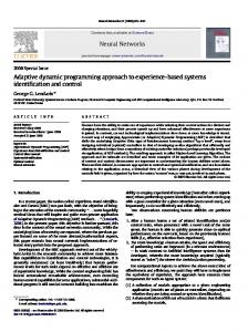
The paper proposes a general framework which encompasses the training of neural networks and the adaptation of filters. We show that neural networks can be considered as general non-linear filters

the adaptive training of neural networks; we first consider transversal filters, whose training is relatively straightforward; we subsequently consider the training of feedback networks for non-linear

which can be trained adaptively, i. e. which can undergo continual training with a possibly infinite number of time-ordered examples. We introduce the canonical form of a neural network. This

recursive adaptive filtering, which is a much richer problem; we introduce undirected, semi-directed, and directed algorithms, and put them into the perspective of standard approaches in adaptive

canonical form permits a unified presentation of network architectures and of gradient-based training algorithms for both feedforward networks (transversal filters) and feedback networks (recursive filters). We show that several algorithms used classically in linear adaptive filtering, and some

filtering (output error and equation error approaches) and adaptive control (parallel and seriesparallel approaches), as well as of algorithms suggested earlier for the training of neural networks.

algorithms suggested by other authors for training neural networks, are special cases in a general classification of training algorithms for feedback networks.

2 1. SCOPES OF ADAPTIVE FILTERS AND OF NEURAL NETWORKS

specially designed in the case of transversal linear filtering; they are referred to as the recursive least

1.1. ADAPTIVE FILTERS

square (RLS) algorithms and their fast (FRLS) versions [Bellanger 1987, Haykin 1991]. Linear adaptive filters are widely used for system and signal modelling, due to their simplicity, and due to the fact that, in many cases (such as the estimation of gaussian signals), they are optimal.

Adaptive filtering is of central importance in many applications of signal processing, such as the modelling, estimation and detection of signals. Adaptive filters also play a crucial role in system

Despite their popularity, they remain inappropriate in many cases, especially for modelling nonlinear systems; investigations along these lines have been performed for adaptive detection [see for

modelling and control. These applications are related to communications, radar, sonar, biomedical electronics, geophysics, etc.

instance Picinbono 1988], prediction and estimation [see for instance McCannon et al. 1982]. Unfortunately, when dealing with non-linear filters, no general adaptation algorithm is available, so

A general discrete-time filter defines a relationship between an input time sequence {u(n), u(n–1), …} and an output time sequence {y(n), y(n–1), …}, u(n) and y(n) being either uni or

that heuristic approaches are used. By contrast, general methods for training neural networks are available; furthermore, neural

multidimensional signals. In the following, we consider filters having one input and one output. The generalization to multidimensional signals is straightforward. There are two types of filters: (i) transversal filters (termed Finite Impulse Response or FIR filters in

networks are known to be universal approximants [see for instance Hornik et al. 1989], so that they can be used to approximate any smooth non-linear function. Since both the adaptation of filters [Haykin 1991, Widrow and Stearns 1985] and the training of neural networks involve gradient

linear filtering) whose outputs are functions of the input signals only; and (ii) recursive filters

techniques, we propose to build on this algorithmic similarity a general framework which

(termed Infinite Impulse Response or IIR filters in linear filtering) whose outputs are functions both of the input signals and of a delayed version of the output signals. Hence, a transversal filter is defined by:

encompasses neural networks and filters. We do this in such a way as to clarify how neural networks can be applied to adaptive filtering problems.

y(n) = Φ [u(n), u(n-1), ..., u(n-M+1)], (1) where M is the length of the finite memory of the filter, and a recursive filter is defined by y(n) = Φ [u(n), u(n-1), ..., u(n-M+1), y(n-1), y(n-2), ...., y(n-N)] (2) where N is the order of the filter. The ability of a filter to perform the desired task is expressed by a criterion; this criterion may be

1.2. NEURAL NETWORKS The reader is assumed to be familiar with the scope and principles of the operation of neural networks; in order to help clarify the relations between neural nets and filters, the present section presents a broad classification of neural network architectures and functions, restricted to networks

either quantitative, e.g., maximizing the signal to noise ratio for spatial filtering [see for instance Applebaum and Chapman 1976], minimizing the bit error rate in data transmission [see for instance

with supervised training.

Proakis 1983], or qualitative, e.g. listening for speech prediction [see for instance Jayant and Noll 1984]. In practice, the criterion is usually expressed as a weighted sum of squared differences

1.2.1. - Functions of neural networks.

between the output of the filter and the desired output (e.g. LS criterion). An adaptive filter is a system whose parameters are continually updated, without explicit control by

The functions of neural networks depend on the network architectures and on the nature of the input

the user. The interest in adaptive filters stems from two facts: (i) tailoring a filter of given architecture to perform a specific task requires a priori knowledge of the characteristics of the input signal; since this knowledge may be absent or partial, systems which can learn the characteristics of the signal are desirable; (ii) filtering nonstationary signals necessitates systems which are capable of tracking the variations of the characteristics of the signal. The bulk of adaptive filtering theory is devoted to linear adaptive filters, defined by relations (1) and (2), where Φ is a linear function. Linear filters have been extensively studied, and are appropriate for many purposes in signal processing. A family of particularly efficient adaptation algorithms has been

data: network architectures: neural networks can have either a feedforward structure or a feedback structure; -

input data: the succession of input data can be either time-ordered or arbitrarily ordered.

3 Feedback networks (also termed recurrent networks) have been used as associative memories, which

2. STRUCTURE OF NEURAL NETWORKS FOR NON-LINEAR FILTERING

store and retrieve either fixed points or trajectories in state space. The present paper stands in a completely different context: we investigate feedback neural networks which are never left to evolve under their own dynamics, but which are continually fed with new input data. In this context, the

2.1. MODEL OF DISCRETE-TIME NEURON

purpose of using neural networks is not that of storing and retrieving data, but that of capturing the (possibly non-stationary) characteristics of a signal or of a system. Feedforward neural networks have been used basically as classifiers for patterns whose sequence of presentation is not significant and carries no information, although the ordering of components within an input vector may be significant. In contrast, the time ordering of the sequence of input data is of fundamental importance for filters: the input vectors can be, for instance, the sequence of values of a sampled signal. At time n, the network is presented with a window of the last M values of the sampled signal {u(n), u(n-1), ..., u(nM+1)}, and, at time n+1, the input is shifted by one time period {u(n+1), u(n), ..., u(n-M+2)}. In this context, feedforward networks are used as transversal filters, and feedback networks are used as recursive filters. A very large number of examples of feedforward networks for classification can be found in the literature. Neural network associative memories have also been very widely investigated [Hopfield 1982, Personnaz 1986, Pineda 1987]. Feedforward networks have been used for prediction [Lapedes and Farber 1988, Pearlmutter 1989, Weigend et al. 1990]. Examples of feedback networks for filtering can be found in [Robinson and Fallside 1989, Elman 1990, Poddar and Unnikrishnan 1991]. Note that the above classification is not meant to be rigid. For instance, Chen et al. [Chen et al. 1990] encode a typical filtering problem (channel equalization) into a classification problem. Conversely,

The behaviour of a discrete-time neuron is defined by relation (3): qij

zi(n) = fi vi (n) = fi

∑ ∑ cij, τ zj(n-τ) j ∈P i

(3)

τ=0

where: fi is the activation function of neuron i, vi is the potential of neuron i, zj can be either the output of neuron j or the value of a network input j, Pi is the set of indices of the afferent neurons and network inputs to neuron i, cij,τ is the weight of the synapse which transfers information from neuron or network input j to neuron i with (discrete) delay τ, qij is the maximal delay between neuron j and neuron i. It should be clear that several synapses can transfer information from neuron (or network input) j to neuron i, each synapse having its own delay τ and its own weight cij,τ . Obviously, one must have cii,0=0 ∀i for causality to be preserved. If neuron i is such that: i ∉ Pi and qij=0 ∀j∈Pi, neuron i is said to be static. 2.2. STRUCTURE OF NEURAL NETWORKS FOR FILTERING

Waibel et al. [Waibel et al. 1989] uses a typical transversal filter structure as a classifier.

The architecture of a network, i.e. the topology of the connections and the distribution of delays, may be fully or partially imposed by the problem that must be solved: the problem defines the sequence

1.2.2. - Non-adaptive and adaptive training .

of input signal values and of desired outputs; in addition, a priori knowledge of the problem may give hints which help designing an efficient architecture (see for instance the design of the

At present, in the vast majority of cases, neural networks are not used adaptively: they are first

feedforward network described in [Waibel et al.1989]). In order to clarify the presentation and to make the implementation of the training algorithms easier,

trained with a finite number of training samples, and subsequently used, e.g. for classification purposes. Similarly, non-adaptive filters are first trained with a finite number of time-ordered samples, and subsequently used with fixed coefficients. In contrast, adaptive systems are trained continually while being used with an infinite number of samples. The instances of neural networks being trained adaptively are quite few [Williams and Zipser 1989a, Williams and Zipser 1989b, Williams and Peng 1990, Narendra and Parthasarathy 1990, Narendra and Parthasarathy 1991].

the canonical form of the network is especially convenient. We first introduce the canonical form of feedback networks; the canonical form of feedforward networks will appear as a special case.

4 2.2.1. - The canonical form of feedback networks

maximum number of external inputs E (M≤E) is done as follows: construct the network graph whose nodes are the neurons and the input, and whose edges are the connections between neurons, weighted

The dynamics of a discrete-time feedback network can be described by a finite-difference equation of order N, which can be expressed by a set of N first-order difference equations involving N

by the values of the delays; find the direct path of maximum weight D from input to output; one has E = D+1. The determination of the order N of the network from the network graph is less straightforward; it is described in Appendix 1.

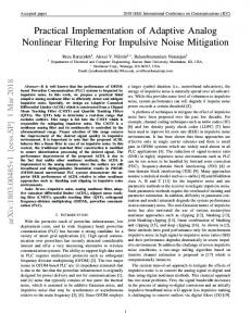
variables (termed state variables) in addition to the M input variables. Thus, any feedback network can be cast into a canonical form which consists of a feedforward (static) network whose outputs are the outputs of the neurons which have desired values, and the values of the state variables, whose inputs are the inputs of the network and the values of the state variables, the latter being delayed by one time unit (Figure 1).

Output at time n

systems investigated in [Narendra 1990]. Figure 2 illustrates the most general form of the canonical form of a network having a single output y(n) and N state variables {y(n-1), ..., y(n-N+1)}. It

.... ....

inputs must be found by trial and error. If we assume that the state variables are delayed values of the output, or if we assume that the state of the system can be reconstructed from values of the input and output, then all state variables have desired values. Such is the case for the NARMAX model [Chen and Billings 1989] and for the

State variables at time n+1

eedforward network

If the task to be performed does not suggest or impose any structure for the filter, one may use either a multi-layer Perceptron, or the most general form of feedforward network in the canonical form, i.e. a fully connected network; in that case, the number of neurons, of state variables and of delayed

...

1

Unit delays

features M external inputs, N feedback inputs and one output; it can implement a fairly large class of functions Φ; the non-recursive part of the network (which implements function Φ ) is a fullyconnected feedforward net.

.......

External network inputs at time n

zM+N+1

State variables at time n

f

f

∑

Figure 1: General canonical form of a feedback neural network.

zM+N+2

∑

zM+N+ ν= y(n)

..

∑

....... 1

Note that the choice of the set of state variables is not necessarily unique: therefore, a feedback

1

1

Fully connected

Unit delays

network may have several canonical forms. The state of the network is the set of values of the state variables. In the following, all vectors will be denoted by uppercase letters. The behaviour of a single-input-single-output network is described by the state equation (4) and output equation (4'): S(n+1) = ϕ[S(n),U(n)]

z1 = u(n)

....

zM= u(n-M+1)

zM+1= y(n-1)

zM+2 = y(n-2)

. . . . . z.

M+N-1= y(n-N+1)

zM+N= y(n-N)

(4)

y(n) = ψ[S(n),U(n)] (4') where U(n) is the vector of the M last successive values of the external input u and S(n) is the vector of the N state variables (state vector). The output of the network may be a state variable. The transformation of a non-canonical feedback neural network filter to its canonical form requires the determination of M and of N. In the single-input-single-output case, the computation of the

Figure 2: Canonical form of a network with a fully-connected feedforward net, whose state variables are delayed values of the output. More specific architectures are described in the literature, implementing various classes of functions ϕ and ψ. Some examples of such architectures are presented in Appendix 2.

5 2.2.2. - Special case: the canonical form of feedforward networks

3.2. ADAPTIVE TRAINING ALGORITHMS

Similarly, any feedforward network with delays, with input signal u, can be cast into the form of a feedforward network of static neurons, whose inputs are the successive values u(n), u(n-1), ..., u(n-

Adaptive algorithms compute, in real time, coefficient modifications based on past information. In the present paper, we consider only gradient-based algorithms, which require the estimation of the

M+1); this puts the network under the form of a transversal filter obeying relation (1): y(n) = Φ [u(n), u(n-1), ..., u(n-M+1)] = Φ [U(n)] .

gradient of the cost function, ∇J(n), and possibly the estimation of J(n); these computations make use of data available at time n.

The transformation of a non-canonical feedforward neural network filter to its canonical form requires the determination of the maximum value M, which is done as explained above in the case of

In the simplest and most popular formulation, a single modification of the vector of coefficients ∆C(n)=C(n)-C(n-1) is computed between time n and time n+1; such a method, usual in adaptive

feedback networks. An example described in Appendix 1 shows that this transformation may introduce the replication of some weights, known as "shared weights".

filtering, is termed a purely recursive algorithm. The modification of the coefficients is often performed by the steepest-descent method, whereby

3. TRAINING ADAPTIVE NEURAL NETWORKS FOR ADAPTIVE FILTERING

∆C(n)=-µ∇J(n). In order to improve upon the steepest-descent method, quasi-Newton methods can be used [Press et al. 1986], whereby ∆C(n)=+µD(n), where D(n) is a vector obtained by a linear transformation of the gradient.

3.1. CRITERION

Purely recursive algorithms were introduced in order to avoid time-consuming computations

The task to be performed by a neural network used as a filter is defined by a (possibly infinite)

between the reception of two successive samples of the input signal. If the application under investigation does not have stringent time requirements, then other possibilities can be considered. For instance, if it is desired to get closer to the minimum of the cost function, several iterations of the

sequence of inputs u and of corresponding desired outputs d. At each sampling time n, an error e(n) is defined as the difference between the desired output d(n) and the actual output of the network y(n): e(n)=d(n)-y(n). For instance, in a modelling process, d(n) is the output of the process to be modelled; in a predictor, d(n) is the input signal at time n+1. The training algorithms aim at finding the network coefficients so as to satisfy a given quality criterion. For example, in the case of non-adaptive training (as defined in Section 1.2.2), the most popular criterion is the Least Squares (LS) criterion; the cost function to be minimized is J(C) = 1 K

K

∑

e(p)2

p=1

Thus, the coefficients minimizing J(C) are first computed with a finite number K of samples; the network is subsequently used with these fixed coefficients. In the context of adaptive training, taking into account all the errors since the beginning of the optimization does not make sense; thus, one can implement a forgetting mechanism. In the present paper, we use a rectangular "sliding window" of length Nc; hence the following cost function: J(n, C) = 1 2

n

∑

e(p)2 .

p=n- Nc+1

The choice of the length Nc of the window is task-dependent, and is related to the typical time scale of the non-stationarity of the signal to be processed. In the following, the notation J(n) will be used instead of J(n, C). The computation of e(p) will be discussed in sections 3.3 and 3.4.2.

gradient algorithm can be performed between time n and time n+1. In that case, the coefficientmodification vector ∆C(n) is computed iteratively as: ∆C(n) = CKn(n) - C0 (n) where Kn is the number of iterations at time n, with Ck(n) = Ck-1(n) + µkDk-1 (n) computed at iteration k-1,

(k=1 to K n), where Dk-1(n) is obtained from the coefficients

and C0(n) = CKn-1 (n-1) . If K n >1, the tracking capabilities of the system in the non-stationary case, or the speed of convergence to a minimum in the stationary case, may be improved with respect to the purely recursive algorithm. The applicability of this method depends specifically on the ratio of the typical time scale of the non-stationarity to the sampling period. As a final variant, it may be possible to update the coefficients with a period T>1 if the time scale of the non-stationarity is large with respect to the sampling period: C0 (n) = CKn-T (n-T) . Whichever algorithm is chosen, the central problem is the estimation of the gradient, ∇ J(n): n ∂J(n) ∂ 1 e(p)2 . = ∑ ∂cij ∂cij 2 p=n- Nc+1 At present, two techniques are available for this computation: the forward computation of the gradient and the popular backpropagation of the gradient. i) The forward computation of the gradient is based on the following relation:

6 n

∂J(n) ∂y(p) = - ∑ e(p) . ∂cij ∂cij p=n- Nc+1

With this notation, the cost function taken into account for the modification of the coefficients at

The partial derivatives of the output at time n with respect to the coefficients appearing on the righthand side are computed recursively in the forward direction, from the partial derivatives of the inputs

J(n) = 1 2

to the partial derivatives of the outputs of the network. ii) In contrast, backpropagation uses a chain derivation rule to compute the gradient of J(n). The required partial derivatives of the cost function J(n) with respect to the potentials are computed in the backward direction, from the output to the inputs. The advantages and disadvantages of these two techniques will be discussed in sections 3.3 and 3.4.2. In the following, we show how to compute the coefficient modifications for feedforward and feedback neural networks, and we put into perspective the training algorithms developed recently for

time n becomes: Nc

∑

em(n) 2

where em(n) = d(n-Nc+m) - ym(n) is the error for block m

computed at time n. As mentioned in section 3.2, two techniques are available for computing the gradient of the cost m=1

function: the forward computation technique (used classically in adaptive filtering) and the backpropagation technique (used classically for neural networks) [Rumelhart et al. 1986]. Thus, each block, from block m=1 to block m=Nc , computes a partial modification ∆cijm of the coefficients and the total modification, at time n, is: Nc

∆cij (n) =

∑

m ∆cij (n) ,

m=1

as illustrated in Figure 3.

neural networks and the algorithms used classically in adaptive filtering. U1 (n-1)

u(n-3) C(n-2)

u(n-M-2)

We consider purely recursive algorithms (i.e. T=1 and Kn=1).The extension to non-purely recursive algorithms is straightforward. As shown in section 2.2.2, any discrete-time feedforward neural network can be cast into a

d(n-1)

C(n-2)

u(n-M-1)

Block 3 C(n-2)

∆cij(n-1) = ∆c1ij(n-1) + ∆c2ij(n-1) + ∆c3ij(n-1) cij(n-1) = cij(n-2) + ∆cij(n-1)

u(n-M)

∆cij2(n-1)

∆cij1(n-1)

U 1(n)

d(n-2)

u(n-2)

∆cij3(n-1)

U 2(n)

d(n-1)

u(n-1) Block 1 C(n-1)

U 3(n)

d(n)

u(n) Block 2 C(n-1)

Block 3

∆cij(n) = ∆c1ij(n) + ∆c2ij(n) + ∆c3ij(n) cij(n) = cij(n-1) + ∆cij(n)

n

∑

e(p)2

p=n- Nc+1

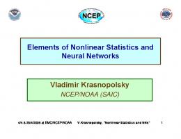
is a sum of Nc independent terms. Its gradient can be computed, from the Nc+M+1 past input data and the N c corresponding desired outputs, as a sum of Nc independent terms: therefore, the modification of the coefficients, at time n, is the sum of Nc elementary modifications computed from Nc independent, identical elementary blocks (each of them with coefficients C(n-1)), between time n and time n+1. We introduce the following notation, which will be used both for feedforward and for feedback networks: the blocks are numbered by m; all values computed from block m of the training network will be denoted with superscript m. For instance, ym(n) is the output value of the network computed by the m-th block at time n: it is the value that the output of the filter would have taken on, at time nNc+m, if the vector of coefficients of the network at that time had been equal to C(n-1).

∆cij1(n)

∆cij2(n)

At time n

C(n-1)

u(n-M+1)

u(n-M)

u(n-M-1)

At time n-1

....

J(n) = 1 2

Block 2

....

previous times. Therefore, the cost function

U 3(n-1)

u(n-1)

....

canonical form in which all neurons are static. The output of such a network is computed from the M past values of the input, and the output at time n does not depend on the values of the output at

d(n-2)

....

Block 1

....

ADAPTIVE FILTERING.

U 2(n-1)

u(n-2)

....

3.3. TRAINING FEEDFORWARD NEURAL NETWORKS FOR NON-LINEAR TRANSVERSAL

d(n-3)

∆cij3 (n)

Figure 3: Computation of two successive coefficient modifications for a non-linear transversal filter (N c=3). It was mentioned above that either the forward computation method or the backpropagation method can be used for the estimation of the gradient of the cost function. Both techniques lead to exactly the same numerical results; it has been shown [Pineda 1989] that backpropagation is less computationally expensive than forward computation. Therefore, for the training of feedforward networks operating as non-linear transversal filters, backpropagation is the preferred technique for gradient estimation. However, as we shall see in the following, this is not always the case for the training of feedback networks. 3.4. TRAINING FEEDBACK NEURAL NETWORKS FOR NON-LINEAR RECURSIVE ADAPTIVE FILTERING.

7

This section is devoted to the adaptive training of feedback networks operating as recursive filters. This problem is definitely richer, and more difficult, than the training of feedforward networks for adaptive transversal filtering. We present a wide variety of algorithms, and elucidate their relationships to adaptation algorithms used in linear adaptive filtering and to neural network training algorithms.

External inputs Um(n)

d(n-Nt +m)

Training block m at time n -

State inputs Sm in (n)

Canonical FF net (non linear)

y

+

m

State outputs m Sout (n)

cm ij , f i

3.4.1. - General presentation of the algorithms for training feedback networks: zm i

Since the state variables and the output of the network at time n depend on the values of the state variables of the network at time n-1, the computation of the gradient of the cost function requires the

f' i

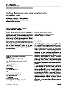
computation of partial derivatives from time n=0 up to the present time n. This is clearly not practical, since (i) the amount of computation would grow without bound, and (ii) in the case of nonstationary signals, taking into account the whole past history does not make sense. Therefore, the estimation of the gradient of the cost function is performed by truncating the computations to a fixed number of sampling periods Nt into the past. Thus, one has to use Nt computational blocks (defined below), numbered from m=1 to m=Nt : the outputs ym (n) are computed through Nt identical versions of the feedforward part of the canonical form of the network (each of them with coefficients C(n-1)). Clearly, Nt must be larger than or equal to Nc in order to compute the Nc last errors em(n). Here again, we first consider the case where T=1 and Kn=1. Figure 4 shows the m-th computational block for the forward computation technique: the state input vector is denoted by S in m (n); the state output vector is denoted by Sout m (n). The canonical feedforward (FF) net computes the output from the external inputs Um (n) and the state inputs Sin m (n). The Forward Computation (FC) net computes the partial derivatives required for the coefficient modification, and the partial derivatives of the state vector which may be used by the next block. The Nt blocks compute sequentially the Nt outputs {ym } and the partial derivatives {∂ym/∂cij}, in the forward direction (m=1 to Nt). The Nc errors {em} (computed from the outputs of the last Nc blocks), and the corresponding partial derivatives are used for the computation of the coefficient modifications, which is the sum of Nc terms: ∆cij (n) = - µ

Nt

Nt

∂J(n) ∂ym =µ ∑ em = ∆cm ij (n) . ∂cij m=N∑ ∂cij m=Nt-Nc+1 t-Nc+1

Details of the computations are to be found in Appendix 3.

FC net (linear) f' i (vm i )

em ∂y m ∂cij

Products

m cm ij , f' i (v i )

∂Sinm ∂cij

m ∂S out (n) ∂cij

(n)

m ∆cm ij (n) = µ e

∂y m ∂cm ij

Figure 4: Training block m at time n with a desired output value: computation of a partial coefficient modification using the forward computation of the gradient for a feedback neural network. If the ouput of block m has no desired value, it has no "products" part and does not contribute directly to coefficient modifications: it just transmits the state variables and their derivatives to the next block.

In order for the blocks to be able to perform the above computations, the values of the state inputs Sinm(n) and of their partial derivatives with respect to the weights must be determined. The choice of these values is of central importance; it gives rise to four families of algorithms.

8 3.4.2. - Choice of the state inputs and of their partial derivatives. 3.4.2.1. - Choice of the state inputs: C(n-1)

C(n-1) C(n-1)

The most "natural "choice of the state inputs of block m is to take the values of the state variables computed by block m-1: Sinm(n)=Soutm-1(n) with Sin1(n)=Sout1(n-1). Thus, the trajectory of the network in state space, computed at time n, is independent of the trajectory of the process: the input of block m is not directly related to the actual values of the state variables of the process to be

n-4

e2

n-3 n-2

e3

modelled by the network, hence the name undirected algorithm. If the coefficients are mismatched, this choice may lead to large errors and to instabilities. Figure 5a shows pictorially the desired

n-1

use the forward computation technique to compute the coefficient modifications (Figure 5b). This choice of the state inputs has been known as the output error approach in adaptive filtering and as the parallel approach in automatic control. It does not require that all state variables have desired

Computed ouput values

Initialization of the partial derivatives

Desired outputs

Computed partial derivatives

(a)

values. In order to reduce the risks of instabilities, an alternative approach may be used, called a semidirected algorithm. In this approach, the state of the network is constrained to be identical to the desired state for m=1: Sinm (n)=Soutm-1(n) with Sin1 (n) = [d(n-Nt), d(n-Nt-1), ..., d(n-Nt-M+1)]. This is possible only when the chosen model is such that desired values are available for all state variables; this is the case for the NARMAX model. Figure 6a shows pictorially the desired trajectory of the state of the network and the trajectory which is computed at time n when a semi-directed algorithm is used (Nt=4, Nc =2). We show in section 3.4.2.2 that, in that case, one can use the backpropagation technique to compute the coefficient modifications (Figure 6b).

Block 1 C(n-1) 1 (n-1) Sout

1 ∂Sout (n-1) ∂cij

technique to compute the coefficient modifications (Figure 7b). In directed algorithms, all blocks are independent, just as in the case of the training of feedforward networks (section 3.3); therefore, one has Nt = Nc.

Sin1 (n)

d(n-1)

Block 2 C(n-1) 1 (n) S out

1 ∂S in1 ∂Sout (n) (n) ∂cij ∂cij

Sin2 (n)

U 3 (n)

d(n)

Block 3 C(n-1) 2 S out (n)

2 ∂S in2 ∂S out (n) (n) ∂cij ∂cij

∆C 2 (n)

Sin3 (n)

3 (n) Sout

3 ∂Sin3 ∂S out (n) (n) ∂cij ∂cij

∆C 3 (n)

(b)

With this choice, the training is under control of the desired values, hence of the process to be

process is less severe than in the previous cases. Figure 7a shows pictorially the desired trajectory of the state of the network and the trajectory which is computed at time n when a directed algorithm is used (N t= Nc=3). We show in section 3.4.2.2 that, in that case, one can use the backpropagation

U 2 (n)

U 1 (n)

The trajectory of the state of the network can be further constrained by choosing the state inputs of all blocks to be equal to their desired values: Sinm(n) = [d(n-Nt+m-1), d(n-Nt+m-2), ..., d(n-Nt+m-M)] for all m. modelled, at each step of the computations necessary for the adaptation (hence the name directed algorithm); therefore, it can be expected that the influence of the mismatch of the model to the

n

Initialization of the feedback inputs

trajectory of the state of the network and the trajectory which is computed at time n when an undirected algorithm is used (Nt=3, Nc=2). We show in section 3.4.2.2 that, in that case, one must

a) b)

Figure 5: Undirected algorithm (with Nt=3 and Nc=2). Pictorial representation of the desired trajectory, and of the trajectory computed at time n, in state space; the trajectory at time n is computed by the blocks shown on Figure 5b. Computational system at time n. The detail of each block is shown on Figure 4. Note that the output of block 1 has no desired value.

9

C(n-1)

C(n-1)

n-5

C(n-1) C(n-1)

n-3

n-4

C(n-1)

e3

n-2

n-4

Output value

U 2 (n)

D1 (n)

Sin1 (n)

1 (n) S out

∂J

(n) 1 ∂ S out

∆ C 1 (n)

d(n-1)

∂J ∂ S2 in

(n)

∂J 2 ∂ Sout

U 4 (n)

Block 3 C(n-1)

2 S out (n)

(n)

∆C 2 (n)

e3

Output value

Block 2 C(n-1) 2 S in (n)

C(n-1)

n-1 U3 (n)

Block 1 C(n-1)

e2

n-2

(a) U 1 (n)

n-3

n-5

n

Desired output value

C(n-1)

e1

e4

n-1

3 S in (n)

3 S out (n)

∂J

Block 4 C(n-1) 4 S in (n)

∂J

n

Desired output value (a)

d(n)

U 1 (n)

d(n-2)

U 2 (n)

d(n-1)

U 3 (n)

d(n)

4 S out (n)

Block 1 C(n-1)

∂J (n) (n) ∂S3 ∂ S3 in out

4 ∂ Sin

∆ C 3 (n)

∆ C 4 (n)

Block 2 C(n-1)

Block 3 C(n-1)

(n)

D1 (n)

Sin1 (n)

D2 (n)

Sin2 (n)

BPnet

BPnet

D3(n)

Sin3 (n)

BPnet

(b) Figure 6: Semidirected algorithm (with Nt=4 and Nc=2). a) Pictorial representation of the desired trajectory, and of the trajectory computed at time n, in state space; the trajectory at time n is computed by the blocks shown on Figure 6b. b) Computational system at time n. The detail of each block is shown on Figure 8. Note that the outputs of blocks 1 and 2 have no desired values, but do contribute an additive term to the coefficient modifications. This choice of the values of the state inputs has been known as the equation error approach in adaptive filtering and as the series-parallel approach in automatic control. It is an extension of the teacher forcing technique [Jordan 1985] used for neural network training. If some state inputs do not have desired values, hybrid versions of the above algorithms can be used: those state inputs for which no desired values are available are taken equal to the corresponding computed state variables (as in an undirected algorithm), whereas the other state inputs may be taken equal to their desired values (as in a directed or in a semi-directed algorithm).

∆C 1 (n)

∆C 2 (n)

∆C 3 (n)

(b) Figure 7: Directed algorithm (with Nt=Nc=3). a) Pictorial representation of the desired trajectory, and of the trajectory computed at time n, in state space; the trajectory at time n is computed by the blocks shown on Figure 7b. b) Computational system at time n. The detail of each block is shown on Figure 8. Note that, in a directed algorithm, each block is independent from the others and must have a desired output value.

10 3.4.2.2. - Consistent choices of the partial derivatives of the state inputs: The choices of the state inputs lead to corresponding choices for the initialization of the partial derivatives, as illustrated in Figures 5a, 6a, 7a. In the case of the undirected algorithm, one has Sinm(n)=Soutm-1(n); therefore, a consistent choice of the values of the partial derivatives of the state inputs consists in taking the values of the partial derivatives of the state outputs computed by the previous block: m-1 ∂Sm in (n) = ∂S out (n) , ∂cij ∂cij except for the first block where one has: ∂S1in (n) ∂S1out (n-1) = . ∂cij ∂cij

Initialization: state input of the first block

Sm in (n) =

S1out (n-1)

S m-1 out (n)

UD-D Algorithm

S1out (n-1)

S m-1 out (n)

zero

UD-SD Algorithm

S1out (n-1)

S m-1 out (n)

zero

Undirected (UD) Algorithm (Output Error) (Parallel)

∂S1out (n-1) ∂cij

Partial derivatives for a current block ∂Sm in (n) = ∂cij ∂Sm-1 out (n) ∂cij

zero

m-1

Initialization: state input of the first block

derivatives can consistently be taken equal to zero. The values of the partial derivatives of the state inputs are taken equal to the values of the partial derivatives of the state outputs computed by the

State input of a current block

Initialization: partial derivatives for the first block ∂S1in (n) = ∂cij

∂S out (n) ∂cij

Partial derivatives for a current block

S1in (n) =

Sm in (n) =

Semi-Directed (SD) Algorithm

Desired values

Sm-1 out (n)

zero

SD-D Algorithm

Desired values

Sm-1 out (n)

zero

SD-UD Algorithm

Desired values

Sm-1 out (n)

∂S1out (n-1) ∂cij

State input of a current block

Initialization: partial derivatives of the first block

Partial derivatives for a current block

S1in (n) =

Sm in (n) =

∂S1in (n) = ∂cij

∂Sm in (n) = ∂cij

Directed Algorithm (D) (Equation Error) (Teacher Forcing) (Series Parallel)

Desired values

Desired values

zero

zero

D-SD Algorithm

Desired values

Desired values

zero

∂S out (n) ∂cij

D-UD Algorithm

Desired values

Desired values

The parameters T, K n, Nt, Nc being fixed, the first three algorithms described above are summarized on the first line of each section of Table 1. The first part of the acronyms refers to the choice of the state inputs and the second part refers to the choice of the partial derivatives of the state inputs. They include algorithms which have been used previously by other authors: the "Real-Time Recurrent

Initialization: partial derivatives for the first block ∂S1in (n) = ∂cij

S1in (n) =

In the case of the semi-directed algorithm, the state input values of the first block are taken equal to the corresponding desired values; the latter do not depend on the coefficients; therefore, their partial

previous block. In the case of the directed algorithm, one can consistently take the partial derivatives of the state inputs of all blocks equal to zero.

State input of a current block

∂Sm in (n) = ∂cij m-1

∂S out (n) ∂cij

zero

∂Sm-1 out (n) ∂cij

Learning Algorithm" [Williams and Zipser 1989a] is an undirected algorithm (using the forward computation technique) with N t=Nc=1. This algorithm is known as the Recursive Prediction Error algorithm, or IIR-LMS algorithm, in linear adaptive filtering [Widrow and Stearns 1985]. The "Teacher-Forced Real-Time Recurrent Learning Algorithm" [Williams and Zipser 1989a] is a hybrid algorithm with Nt=Nc=1.

Initialization: state input of the first block

m-1

∂S1out (n-1) ∂cij

∂Sm-1 out (n) ∂cij

Table 1: Three families of algorithms for the training of feedback neural networks. In each section, the first line describes the algorithms with consistent choices of the state inputs (sec. 3.4.2.2).

11

The above algorithms have been introduced in the framework of the forward computation of the gradient of the cost function. However, the estimation of the gradient of the cost function by backpropagation is attractive with respect to computation time, as mentioned in section 3.3.4. If this technique is used, the computation is performed with Nt blocks, where each coefficient cij is replicated in each block m as cijm. Therefore, one has: ∂vm i = zm . j ∂cm ij The training block m is shown in Figure 8: after computing the Nc errors using the Nt blocks in the forward direction, the Nt blocks compute the derivatives of J(n) with respect to the potentials {vim}, in the backward direction. The modification of the coefficients is computed from the Nt blocks as: Nt Nt ∂J(n) m ∂J(n) ∆cij (n) = - µ =µ ∑ zj = ∑ ∆cm ij (n) . m ∂cij m=1 ∂vi m=1

d(n-Nt +m) External inputs Um(n)

Training block m at time n

ym

(non linear)

State outputs m S out (n)

cm ij , fi zm i

BP net

can be found in [Narendra and Parthasarathy 1990]. 3.4.2.3. - Other choices of the partial derivatives of the state inputs: Because adaptive neural networks require real-time operation, tradeoffs between consistency and computation time may be necessary: setting partial derivatives ∂Sinm/∂cij equal to zero may save time by making the computation by backpropagation possible even for undirected algorithms (UD-D line shows the characteristics of the fully consistent algorithm, whereas the other two lines show other possibilities which are not fully consistent, but which can nevertheless be used with advantage. The SD-UD, D-SD and D-UD algorithms have been included for completeness: computation time permitting, the accuracy of the computation may be improved by setting the partial derivatives of the

algorithm with N c =1 and Nt>1, with a special feature: in order to save computation time, the coefficients of the blocks 1 to Nt-1 are the coefficients which were computed at the corresponding

em

(linear) m cm ij , f i' (vi )

∆ cm ij (n) = - µ

backpropagation is the best choice because of its lower computational complexity. An example of the use of a directed algorithm for idenfication and control of non-linear processes

UD-D algorithm with Nt=2, Nc=1 [Shynk 1989]. The truncated backpropagation through time algorithm [Williams and Peng 1990] is a UD-D

f i'( vm i )

Products

∂J ∂S m in

algorithms (Figures 6b and 7b); backpropagation cannot be used consistently within undirected and hybrid algorithms. When both backpropagation and forward computation techniques can be used,

state inputs to non-zero values in the directed or semi-directed case. Undirected algorithms have been in use in linear adaptive filtering: the extended LMS algorithm is a UD-D algorithm (see table 1) with Nt=Nc=1 [Shynk 1989]; the a posteriori error algorithm is also a

f i'

∂J ∂vim

lead to the same coefficient modifications as the forward propagation technique if and only if it is used within algorithms complying with this condition, i.e. within directed or semi-directed

or UD-SD algorithms). The full variety of algorithms is shown on Table 1: in each group, the first -+

Canonical FF net State inputs Sm in (n)

It is important to notice that backpropagation assumes implicitly that the partial derivatives of the state inputs of the first copy are taken equal to zero. Therefore, the backpropagation technique will

∂J ∂S m out

∂J m zj ∂vim

Figure 8: Training block m at time n with a desired output value: computation of a partial coefficient modification using the backpropagation technique for the estimation of the gradient for a feedback neural network. If block m has no desired value, then em=0, but it does contribute an additive term to the coefficient modification. It should be noticed that forward propagation through all blocks must be performed before backpropagation.

times.

12 CONCLUSION APPENDIX 1 The present paper provides a comprehensive framework for the adaptive training of neural networks, viewed as non-linear filters, either transversal or recursive. We have introduced the concept of

We consider a discrete-time neural network with any arbitrary structure, and its associated network

canonical form of a neural network, which provides a unifying view of network architectures and allows a general description of training methods based on gradient estimation. We have shown that

graph as defined in section 2.2. The set of state variables is the minimal set of variables which must be initialized in order to allow

backpropagation is always advantageous for training feedforward networks adaptively, but that it is not necessarily the best method for training feedback networks. In the latter case, four families of

the computation of the state of all neurons at any time n>0, given the values of the external inputs at all times from 0 to n. The order of the network is the number of state variables.

training algorithms have been proposed; some of these algorithms have been in use in classical linear adaptive filtering or adaptive control, whereas others are original.

Clearly, the only neurons whose state must be initialized are the neurons which are within loops (i.e. within cycles in the network graph). Therefore, in order to determine the order of the network, the

The unifying concepts thus introduced are helpful in bridging the gap between neural networks and adaptive filters. Furthermore, they raise a number of challenging problems, both for basic and for applied research. From a fundamental point of view, general approaches to the convergence and

network graph should be pruned by suppressing all external inputs and all edges which are not within cycles (this may result in a disconnected graph). To determine the order, it is convenient to further simplify the network graph as follows: (i) merge

stability of these algorithms are still lacking; a preliminary study along these lines has been presented

parallel edges into a single edge whose delay is the maximum delay of the parallel edges; (ii) if two

[Dreyfus et al. 1992]; from the point of view of applications, the real-time operation of non-linear adaptive systems requires specific silicon implementations, thereby raising the questions of the speed and accuracy required for the computations.

edges of a loop are separated by a neuron which belongs to this loop only, suppress the neuron and merge the edges into a single edge whose delay is the sum of the delays of the edges. We now consider the neurons which are still represented by nodes in the simplified network graph. We denote by N the order of the network.

ACKNOWLEDGEMENTS The authors are very grateful to O. MACCHI for numerous discussions which have been very

If, for each node i of the simplified graph, we denote by Ai the delay of the synpase, afferent to neuron i, which has the largest delay (i.e. the weight of the edge directed towards i which has the

helpful in putting neural networks into the perspective of adaptive filtering. C. VIGNAT has been instrumental in formalizing some computational aspects of this work. We thank H. GUTOWITZ for

largest weight), then a simple upper bound for N is given by: N ≤ Σi Ai .

his critical reading of the manuscript.

The state xi of a neuron i which has an afferent synapse of delay Ai cannot be computed at times n 0 ,

ωi = 0 otherwise, where Ri stands for the set of indices of the nodes which are linked to i by an edge directed from i to j (i.e. the set of neurons to which neuron i projects efferent synapses). Then the order of the network is given by: N= Σi ωi . The necessity of imposing the state of neuron i at time k (0