Third International Conference on CFD in the Minerals and Process Industries CSIRO, Melbourne, Australia 10-12 December 2003
NUMERICAL SIMULATION OF VISCOUS FLOW OF A NON-NEWTONIAN FLUID PAST AN IRREGULAR SOLID OBSTACLE BY THE MIRROR FLUID METHOD Chao YANG and Zai-Sha MAO Institute of Process Engineering, Chinese Academy of Sciences, Beijing 100080, China Email:
[email protected] (C. Yang),
[email protected] (Z.-S. Mao)
the inner surface of the pipe is considered. It is a difficult problem for theoretical analysis, but nowadays various rapidly developing computational fluid dynamics approaches allow us to solve this problem numerically.
ABSTRACT The mirror fluid method is proposed for simulating viscous tubular flow of a Newtonian or non-Newtonian fluid past an irregular solid obstacle using a simple finite difference method for discretization. Suitable flow parameters in the solid domain are assigned by a mirror relation to ensure the surface segment is subjected to zero net shear and normal forces and the boundary conditions are enforced implicitly on the solid-fluid surface. The SIMPLE scheme and the control volume formulation are used for solving the governing equations and a 5th order weighted ENO scheme is adapted for discretization of the constitutive equations. Some typical numerical examples including Newtonian, power-law, Carreau-Bird and Oldroyd-B fluids past half-circular, triangular or trapeziform obstacles in a straight tube are simulated successfully in a two-dimensional axisymmetric coordinate system.
This problem of flow past an irregular solid obstacle, especially for a viscoelastic fluid, is scarcely simulated, perhaps due to the involved irregular solid surfaces. The abrupt change of geometry with singularities may cause very high levels of stress, and in turn enhance numerical instabilities for a viscoelastic fluid and lead to divergence at high Deborah numbers (Dou and Phan-Thien, 1999). Many finite element methods have been proposed to deal with fluid flow, with the advantage of easily generated triangular meshes fitted propagating irregular interfaces, and was adopted by most reported numerical studies on non-Newtonian flow past a sphere or a cylinder, annular flow between two eccentric cylinders, and the sedimentation or fluidization of a single and hundreds of solid particles (Aboubacar et al., 2002; Caola et al., 2001; Fan et al., 1999; Glowinski et al., 2001; Huang et al., 1998; Missirlis et al., 2001; Patankar et al., 2001; Singh et al., 2000; Smith et al., 2003). The finite element method is generally more intricate and requires a larger amount of computer memory space than the finite difference method. Also the continuity equation is not easy to be satisfied for incompressible fluids.
NOMENCLATURE A configuration tensor g gravitational acceleration, m·s-2 p pressure, Pa r radial coordinate, m t time, s u velocity vector, m·s-1 u axial velocity component, m·s-1 v radial or transverse velocity component, m·s-1 x axial coordinate, m y radial or transverse coordinate, m φ level set function µ viscosity, Pa·s ρ density, kg·m-3
Since a regular Eulerian grid is not easy for computation of solid-fluid flow with irregular solid surfaces by finite differences, an orthogonal, boundary-fitted coordinate system (Ryskin and Leal, 1983) or the unstructured finite volume method (Prakash and Patankar, 1984) can be applied to model some free or irregular boundary problems with good accuracy in enforcing the boundary conditions (Dou and Phan-Thien, 1998, 1999; Mao, 2002; Mao and Chen, 1997; Missirlis et al., 2001). However, it is very difficult to construct the orthogonal curvilinear coordinates or boundary-fitted adaptive meshes for complicated and seriously deformed interfaces, e.g., the tubular flow past a half-circular obstacle on the inner wall. Inspired by the fictitious domain method (Glowinski et al., 2001; Singh et al., 2000) and the ghost fluid method (Fedkiw, 2002; Fedkiw et al., 1999), we have accordingly developed a novel computational method (Yang and Mao, 2003), i.e., the mirror fluid method, for numerical simulation of the sedimentation of a solid particle in a Newtonian fluid on a regular Eulerian grid. The Reynolds number, drag coefficient and wake length of a falling sphere were well predicted as verified against the acknowledged experimental data. In this novel algorithm, suitable flow parameters are assigned to the solid domain
Subscripts
x y
θ
axial direction radial or transverse direction azimuthal direction
INTRODUCTION The viscous channel flow of a Newtonian or nonNewtonian fluid past a solid protuberance is significant to many process industry applications. Different methods such as experimental, mathematical analyses or numerical simulation can be employed for studying the process fluid flow. Here the tubular flow of a shear thinning generalized Newtonian or viscoelastic fluid in a straight pipe with half-circular, triangular or trapeziform solid obstacles on
Copyright © 2003 CSIRO Australia
391
by a mirror relation to ensure the boundary conditions are accurately enforced on solid-fluid surface segments. This algorithm has the advantages of using a simple finite difference method for discretization and adopting a fixed Cartesian grid without need of re-meshing.
∇
τ=
∇
(9) τ Ε + λ1 τ Ε = 2 µ E D Here λ1 and λ2 are characteristic relaxation and retardation times for the viscoelastic fluid, respectively, and the fluid reduces to a Newtonian fluid when λ1 = λ2 and to an upper convected Maxwell model when λ1 ≠ 0 and λ2 = 0 . The fluid viscosity µ = µ N + µ E , where µ N is the purely viscous contribution to viscosity and µ E = cµ N is the viscosity of the viscoelastic contribution and c = λ1 λ2 − 1 .
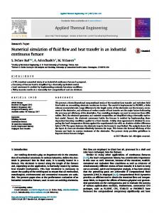
GOVERNING EQUATIONS To demonstrate and validate the applicability of the mirror fluid method for the simulation of a non-Newtonian fluid flow past an irregular solid surface, the laminar flow of a generalized Newtonian fluid or an Oldroyd-B viscoelastic fluid in an axisymmetric tube is considered. As shown in Fig. 1, three typical kinds of solid obstacles are considered: half-circular, triangular or trapeziform obstacles clinging around on the inner wall of a straight tube, where Rb is the radius of the half-circular obstacle, and W and H are the underside width and height of the isosceles triangular or trapeziform obstacle, respectively. The mass and momentum conservation equations for an incompressible fluid can be written as (1)
∂u + u ⋅ ∇ u = −∇ p + ρ g + ∇ ⋅ τ ∂t
(2)
ρ
(
)
(a) A half-circular obstacle
W=2Rb H
y (v )
(b) An isosceles triangular obstacle ( H = 0.8Rb )
W=3Rb H
y (v )
Rb
Rt
x (u )
τ = µ γ&
(4) where γ& is the strain rate defined in terms of the deformation tensor D , i.e., γ& = 2 D : D , and the viscosity
(c) An isosceles trapeziform obstacle ( H = 0.8Rb ) Figure 1: A schematic diagram of a straight tube with a solid obstacle on inner wall.
µ varies according to the power-law model:
(5) In a two-dimensional axisymmetric coordinate system, the continuity and Navier-Stokes equations and the constitutive equation (9) for the Oldroyd-B model in terms of configuration tensor can be written in component form:
or is given by the Carreau-Bird law:
(
)
n −1 µ − µ∞ (6) = 1 + ( λ3 γ& ) 2 2 µ0 − µ∞ where k is the consistency index, n is a parameter between 0 and 1 for shear thinning fluids, µ0 is the zero shear viscosity, µ ∞ is the minimum viscosity achieved as shear rate approaches infinity, and λ3 is assumed to be 1. For a viscoelastic fluid, the constitutive equation of Oldroyd-B model is ∇
∂u 1 ∂ (rv ) = 0 + ∂x r ∂y ∂ (ρu ) + ∂ ρuu − µ N ∂u + 1 ∂ rρvu − rµ N ∂u ∂y ∂t ∂x ∂x r ∂y A ∂p ∂ ∂u + ρg x + µ N + c µ N xx ∂x ∂x ∂x λ1 Axy ∂v 1 ∂ rµ N + + rcµN r ∂y ∂x λ1
=−
(7)
τ + λ1 τ = 2 µ(D + λ2 D)
where the upper convected derivative of
Rt
x (u )
(3)
µ = k γ& n −1
Rt
x (u )
The constitutive equation that relates stresses with velocity gradients can be given by the generalized Newtonian model:
∇
Rb
y (v )
where τ is the extra stress tensor and for a Newtonian fluid τ = 2 µ N D . The rate-of-deformation tensor D is defined as D = 1 ∇ u + ∇u T 2
(8)
Let τ Ε = µ E ( A - I ) λ1 = τ - 2µ N D , then Eq. (7) can be written in the form of
In this paper, the mirror fluid method is used to give a comparatively robust and effective finite difference scheme for the tubular flow of a Newtonian and a nonNewtonian fluid, such as power-law, Carreau-Bird model and Oldroyd-B fluids, past a irregular solid protuberance surface in a laminar flow regime.
∇⋅u = 0
∂τ + u ⋅ ∇ τ - ∇u ⋅ τ - τ ⋅ ∇u T ∂t
∇
τ
is defined by
392
(10)
(11)
and can be derived by solving Eqs. (18) and (19) coupled with the condition in Eq. (20):
∂ (ρv ) + ∂ ρuv − µ N ∂v + 1 ∂ rρvv − rµ N ∂v ∂y ∂t ∂x ∂x r ∂y (12) Axy ∂p ∂ ∂u = − + ρg y + µ N + cµN ∂y ∂x ∂y λ1 A A ∂v 1 ∂ 2v yy rµ N − µ + + r cµN + c µ N θθ r ∂y ∂y λ1 N r 2 r λ1 ∂Axx ∂A ∂A ∂u ∂u 1 + u xx + v xx = 2 Axx + 2 Axy − ( Axx − 1) λ1 ∂t ∂x ∂y ∂x ∂y ∂Axy ∂t
+u
∂A yy ∂t
∂Axy ∂x
+u
+v
∂A yy ∂x
∂Axy ∂y
+v
=
∂u ∂v ∂u 1 ∂v Axx + A yy − Axy + Axy + λ1 ∂y ∂x ∂x ∂y
∂A yy ∂y
=2
(
)
1 ∂v ∂v Axy − A −1 A yy + 2 ∂x λ1 yy ∂y
( x M − xS ) 2 + ( y M − yS ) 2 = ( 2φ S ) 2
(19)
φ M φS ≤ 0
(20)
(if φ S ≤ 0 , then φ M ≥ 0 )
(13) (14) (15)
∂Aθθ ∂A ∂A 2v 1 + u θθ + v θθ = Aθθ − ( Aθθ − 1) (16) ∂t ∂x ∂y r λ1 where r ≡ 1 for Cartesian coordinates, r ≡ y for cylindrical
coordinates and curly brackets indicate the term presents only in cylindrical coordinates, and Eq. (16) for the azimuthal normal component of configuration tensor ( Aθθ ) evolution is also needed only in cylindrical coordinates.
Figure 2: Schematic diagram of solid-fluid interface for the mirror fluid method. Then for each node ( S ) in the solid obstacle there is a mirror image node ( M ) in the fluid. The fictitious velocity, pressure and stress of node S in the mirror fluid are obtained easily:
MIRROR FLUID METHOD The detailed idea of the mirror fluid method has been presented by Yang and Mao (2003). We model the whole domain as a regular Eulerian one by taking the flow in the subdomain occupied by the solid obstacle (i.e., the mirror fluid domain) as the flipped mirror image of the outside flow in the real fluid at the same surface segment, i.e., rotating the outside flow field, pressure and stress field by 180 degree around the surface segment (as shown in Fig. 2). Therefore, the shear rates across the solid surface are assigned the same magnitude but with opposite direction to make a surface segment subjected to a zero net force, i.e., the no-slip boundary conditions are enforced implicitly on irregular solid-fluid surface segments by a mirror relation.
u S = −( u M − U ) + U = 2 U − u M
pS = pM
(22)
(23) τS = − τ M where U is the velocity vector of the solid obstacle ( U = 0 for this work), and for a Newtonian or generalized Newtonian fluid we need not apply Eq. (23) to assign the stress. Such specification for flow parameters ensures that the shear and normal stresses on the two sides of the solidfluid interface and endued with the same magnitude and opposite direction. The density and viscosity of the mirror fluid are designated simply equal to those of the corresponding real fluid, i.e., ρ S = ρ M and µ S = µ M . In
As depicted in Fig. 2, we can find the mirror location of M ( x M , y M ) in the real fluid region corresponding to node S ( xS , yS ) in the fictitious domain occupied by the solid obstacle (i.e., the mirror fluid) in terms of a distance function defined similar to that in the level set approach (Yang and Mao, 2002). The signed algebraic distance function denoted as φ , being positive in the fluid phase, negative in the solid phase and zero at the obstacle-fluid interface, to facilitate the mirror calculations. In twodimensional Cartesian or cylindrical coordinates, the unit normal vector passing through node S to the interface is denoted as
this way, we can update the fluid velocity field including the mirror fluid in the entire computational domain with the solid-fluid interface boundary conditions enforced implicitly and with no need of boundary-fitted coordinates. Moreover, it is noted that only a band of several mirror nodes close to the obstacle surface is actually needed by this algorithm. All the nodes in the particle domain whose neighbor nodes are all in the same domain are actually irrelevant to the solution and can be blocked out from the computation as suggested by Patankar (1980).
∇φ n (17) = xS nS = n yS ∇φ S So the coordinates of M , the mirror to S , should agree
COMPUTATIONAL SCHEME No-slip conditions are imposed for velocity on the solid surface. For a fully developed tubular flow, u = v = 0 , ∂u ∂x = ∂v ∂x = 0 , and from the continuity equation ∂v ∂y = 0 . The configuration tensor for the Oldroyd-B model on the solid wall is thus expressed in terms of the velocity gradient through solving the momentum and constitutive equations:
with the following Eq. (18) based the governing equation for the straight line along nS passing through S : x M − xS y M − yS = n xS n yS
(21)
(18)
393
2
Axx = 1 + 2λ12 ∂u , ∂y w
Ayy = 1 ,
number of fully-developed tubular flow without a solid obstacle. The shear thinning of generalized Newtonian fluids increases the Reynolds number and the length of vortex behind the solid obstacle. The mirror fluid method is also used to simulate successfully the viscous flow with other irregular solid surfaces, such as triangular and trapeziform solid protuberance surfaces. The flow field and pressure distribution of a Carreau-Bird law fluid past different obstacles are compared in Figs. 4 and 5. As shown in Figs. 6~9, due to the influence of elasticity the contours of streamline, pressure and velocity for a viscoelastic fluid past a half-circular obstacle in a tube differ obviously from those for a Newtonian or generalized Newtonian fluid. The vortex and the distributions of velocity and pressure are similar to the results for an Oldroyd-B fluid past a cylinder in channel with Re =0 (Dou and Phan-Thien, 1999). Beside the discussion of computational restriction at high Deborah number for a viscoelastic fluid, the effects of Reynolds number, Deborah number and R b R t on the wake length, normal and shear stresses and drag force will be detailed in another paper.
Axy = λ1 ∂u , ∂y w Aθθ = 1
(24)
For a Newtonian fluid, we can directly use the fully developed parabolic velocity distribution as the inflow condition. For a non-Newtonian fluid, on the other hand, the inflow velocity and configuration tensor profile can be obtained by solving the governing equations for a steady flow in a straight tube with a regular and smooth inner wall. The initial value of A is taken as I , implying the Oldroyd-B fluid is in a relaxed state. The control volume formulation with the power-law scheme and the SIMPLE algorithm described by Patankar (1980) are adopted to solve Eqs. (10) to (16) for the fluid. A staggered grid is used and the different dependent variables are approximated at different mesh points. The normal stresses, i.e., Axx , Ayy and Aθθ , are located at the same position as the pressure variables, while the shear stresses, i.e., Axy , at the corners of the control mesh cells for velocities. A 5th order weighted ENO scheme (Fedkiw et al., 1999) for discretization of the constitutive equations (13)~(16) is applied to achieve higher order accuracy in space, and a third-order Runge-Kutta scheme (Yang and Mao, 2002) in time is used to avoid any instability and divergence in the temporal integration of configuration tensors evolution equations. NUMERICAL RESULTS AND DISCUSSION The above-mentioned governing equations are nondimensionalized by introducing characteristic scales and the Reynolds and Deborah numbers are then defined as
Re ≡
ρ dU , µ
De ≡
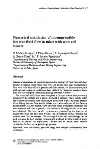
(a) Newtonian fluid ( Re =157.5, Re* =100.0)
λ1U
(25) d where U is the maximum average cross-section velocity in the tube and d is the diameter of the tube ( d = 2Rt ). Typically we solve the tubular flow past a solid obstacle with Rb Rt =0.2 in a computational domain
Ω = {(x, y) 0 ≤ x ≤ 15Rt , − Rt ≤ y ≤ Rt } with the center
of the solid obstacle located at x = 3Rt to assure a fullydeveloped downstream flow. The time step is taken according to the Courant-Friedrich-Lewy conditions and also the restrictions due to viscous terms to make the numerical procedure stable and convergent (Yang and Mao, 2002, 2003). The effect of grid fineness on computations has been investigated. Grids of 93×10, 141×16, 171×20, 186×22, 244×30 and 315×40 are used to test the convergence of the tubular flow by comparing the wake length behind a half-circular obstacle for a nonNewtonian fluid satisfying the Carreau-Bird law with Re =204. The predicted wake length decreases closer to a constant value with the increase of the total number of nodes and a grid with 244×30 is sufficient for spatial computational accuracy. Therefore, the grid of 244×30 is adopted for subsequent simulations.
(b) power-law model fluid ( Re =209.2, Re* =127.5, k =0.1 Pa·s, n =0.8)
(c) Carreau-Bird law fluid ( Re =203.9, Re* =126.2, µ 0 =0.1 Pa·s, µ∞ =0.1 µ 0 , n =0.8)
The streamline contours for Newtonian, power-law and Carreau-Bird fluids past a half-circular obstacle with the same initial inflow velocity ( u =0.01m/s) are presented in
Figure 3: Streamline contours for different fluids past a half-circular obstacle.
Fig. 3, where Re* is the average cross-section Reynolds
394
(a) Triangular obstacle ( Re =177.1, Re* =126.2)
(c) Trapeziform obstacle ( Re =185.3, Re* =126.2) Figure 5: Contours of pressure p for a Carreau-Bird law fluid past different obstacles ( µ 0 =0.1 Pa·s, µ∞ =0.1 µ 0 , n =0.8).
(b) Trapeziform obstacle ( Re =185.3,
Re* =126.2)
Figure 4: Streamline contours for a Carreau-Bird law fluid past non-spherical obstacles ( µ 0 =0.1 Pa·s, µ∞ =0.1µ0, n =0.8).
Figure 6: Streamline contours for an Oldroyd-B fluid past a half-circular obstacle ( De =1.93, c =7, Re =19.8, Re* =12.5).
(a) Half-circular obstacle ( Re =203.9, Re* =126.2)
Figure 7: Contours of pressure p for an Oldroyd-B fluid past a half-circular obstacle ( De =1.93, c =7, Re =19.8, Re* =12.5, Rb Rt =0.2).
(b) Triangular obstacle ( Re =185.3, Re* =126.2) Figure 8: Contours of axial velocity u for an Oldroyd-B fluid past a half-circular obstacle ( De =1.93, c =7, Re =19.8, Re* =12.5).
395
viscosity vorticity (DAVSS-ω) formulation”, J. NonNewtonian Fluid Mech. 87, 47. DOU, H.-S. and PHAN-THIEN, N., (1998), “Parallelisation of an unstructured finite volume code with PVM: viscoelastic flow around a cylinder”, J. NonNewtonian Fluid Mech. 77, 21. FAN, Y., TANNER, R.I. and PHAN-THIEN, N., (1999), “Galerkin/least-square finite-element methods for steady viscoealstic flows”, J. Non-Newtonian Fluid Mech. 84, 233. FEDKIW, R.P., (2002), “Coupling an Eulerian fluid calculation to a Lagrangian solid calculation with the ghost fluid method”, J. Comput. Phys. 175, 200. FEDKIW, R.P., ASLAM, T., MERRIMAN B. and OSHER, S., (1999), “A non-oscillatory Eulerian approach to interfaces in multimaterial flows (the ghost fluid method)”, J. Comput. Phys., 152, 457. GLOWINSKI, R., PAN, T.W., HESLA, T.I., JOSEPH, D.D. and J. PÉRIAUX, (2001), “A fictitious domain approach to the direct numerical simulation of incompressible viscous flow past moving rigid bodies: application to particulate flow”, J. Comput. Phys. 169, 363. HUANG, P.Y., HU, H.H. and JOSEPH, D.D., (1998), “Direct simulation of the sedimentation of elliptic particles in Oldroyd B fluids”, J. Fluid Mech. 362, 297. MAO, Z.-S., (2002), “Numerical simulation of viscous flow through spherical particle assemblage with the modified cell model”, Chinese J. Chem. Eng. 10, 149. MAO, Z.-S. and CHEN, J.Y., (1997), “Numerical solution of viscous flow past a solid sphere with the control volume formulation”, Chinese J. Chem. Eng. 5, 105. MISSIRLIS, K.A., ASSIMACOPOULOS, D., MITSOULIS, E. and CHHABRA, R.P., (2001), “Wall effects for motion of spheres in power-law fluids”, J. NonNewtonian Fluid Mech., 96, 459. PATANKAR, N.A., HUANG, Y., KO, T. and JOSEPH, D.D., (2001), “Lift-off of a single particle in Newtonian and viscoelastic fluids by direct numerical simulation”, J. Fluid Mech. 438, 67. PATANKAR, S.V., (1980), Numerical Heat Transfer and Fluid Flow, Hemisphere, Washington. PRAKASH, C. and PATANKAR, S.V., (1984), “A control volume-based finite-element method for solving the Navier-Stokes equations using equal-order velocitypressure interpolation”, Numerical Heat Transfer 8, 259. RYSKIN, G. and LEAL, L.G., (1983), “Orthogonal mapping”, J. Comput. Phys. 50, 71. SINGH, P., JOSEPH, D.D., HESLA, T., GLOWINSKI, R. and PAN, T.-W., (2000), “A distributed Lagrange multiplier /fictitious domain model for viscoelastic particulate flows”, J. Non-Newtonian Fluid Mech. 91, 165. SMITH, M.D., JOO, Y.L., ARMSTRONG, R.C. and BROWN, R.A., (2003), “Linear stability analysis of flow of an Oldroyd-B fluid through a linear array of cylinders”, J. Non-Newtonian Fluid Mech., 109, 13. YANG, C. and MAO, Z.-S., (2003), “The mirror fluid method for numerical simulation of sedimentation of a solid particle in a Newtonian fluid”, submitted to J. Comput. Phys. (revision under review). YANG, C. and MAO, Z.-S., (2002), “An improved level set approach to the simulation of drop and bubble motion”, Chinese J. Chem. Eng. 10, 263.
Figure 9: Contours of radial velocity v for an Oldroyd-B fluid past a half-circular obstacle ( De =1.93, c =7, Re =19.8, Re* =12.5). CONCLUSION A novel mirror fluid method is presented for numerical simulation of viscous tubular flow of a Newtonian or nonNewtonian fluid past an irregular solid obstacle using a simple finite difference method for discretization. The entire computational domain is modeled as a fixed Eulerian one without using a body-fitted coordinate system and we assign suitable flow parameters in the solid domain by a mirror relation to ensure the surface segment subjected to zero net shear and normal forces. The SIMPLE scheme and the control volume formulation are used for solving the governing equations. Some typical numerical examples including Newtonian, power-law, Carreau-Bird and Oldroyd-B fluids past a half-circular, triangular or trapeziform obstacle fixed on the inner wall of a straight tube are simulated successfully in a twodimensional axisymmetric coordinate system. The vortex and the distributions of velocity and pressure for a viscoelastic fluid differ obviously from those for a Newtonian or generalized Newtonian fluid. These numerical tests indicate the mirror fluid method is simple and effective in simulating viscous flows with irregular solid surfaces. The mirror fluid method can be extended to multiple particle problems with less restriction, especially when complicated and seriously deformed solid-fluid interfaces involved. In future work, the mirror fluid method will be used to compute the motion of a non-spherical (e.g., ellipsoidal and slender) solid particle with rotation or tilting, and multi-particle systems with particle collisions in a Newtonian or non-Newtonian fluid. ACKNOWLEDGMENTS Authors are acknowledged the financial support of the National Natural Science Foundation of China (Nos. 20236050, 20106016) and very grateful to Prof. Jiayong Chen in our institute for his valuable support and advice. REFERENCES ABOUBACAR, M., MATALLAH, H., TAMADDONJAHROMI, H.R. and WEBSTER, M.F., (2002), “Numerical prediction of extensional flows in contraction geometries: hybrid finite volume/element method”, J. Non-Newtonian Fluid Mech., 104, 125. CAOLA, A.E., JOO, Y.L., ARMSTRONG, R.C. and BROWN, R.A., (2001), “Highly parallel time integration of viscoelastic flows”, J. Non-Newtonian Fluid Mech. 100, 191. DOU, H.S. and PHAN-THIEN, N., (1999), “The flow of an Oldroyd-B fluid past a cylinder in a channel: adaptive
396