... in the literature. Index Termsâ Object detection, data fusion, graph cut ... 3D shapes in the real world as point clouds have enabled high- ... high vegetation (green), car (yellow). ... neural networks were used with the RGB and LiDAR gener-.
OBJECT DETECTION USING OPTICAL AND LIDAR DATA FUSION Onur Tas¸ar, Selim Aksoy Department of Computer Engineering Bilkent University Bilkent, 06800, Ankara, Turkey {onur.tasar,saksoy}@cs.bilkent.edu.tr ABSTRACT Fusion of aerial optical and LiDAR data has been a popular problem in remote sensing as they carry complementary information for object detection. We describe a stratified method that involves separately thresholding the normalized digital surface model derived from LiDAR data and the normalized difference vegetation index derived from spectral bands to obtain candidate image parts that contain different object classes, and incorporates spectral and height data with spatial information in a graph cut framework to segment the rest of the image where such separation is not possible. Experiments using a benchmark data set show that the performance of the proposed method that uses small amount of supervision is compatible with the ones in the literature. Index Terms— Object detection, data fusion, graph cut 1. INTRODUCTION Automatic detection of objects such as buildings and trees in very high spatial resolution optical images has been a common task in many applications such as urban mapping, planning and monitoring. However, using only spectral information for object detection may not be sufficiently discriminative because colors of pixels belonging to the same object may have very high variations. In addition, shadows falling onto objects also make the detection task more difficult. More recently, developments in the Light Detection and Ranging (LiDAR) technology and its capability of capturing 3D shapes in the real world as point clouds have enabled highresolution digital surface models (DSM) as additional data sources. Consequently, exploiting both color and height information together by fusing aerial optical and DSM data has been a popular problem in remote sensing image analysis. Both rule-based and supervised learning-based classification of optical and DSM data have been studied in the literature [1]. For example, Moussa and El-Sheimy [2] used height information to separate buildings and trees from the ground, and applied a threshold on the normalized difference vegetation index (NDVI) to separate buildings from trees. This
(a)
(b)
(c)
Fig. 1. An example test area used in this paper. (a) Ortho photo. (b) DSM. (c) Reference data with class labels: impervious surfaces (white), building (blue), low vegetation (cyan), high vegetation (green), car (yellow).
method could identify the visible building and vegetation regions well, but misclassified the vegetation within shadowed areas. To solve this problem, Grigillo and Kanjir [3] empirically defined multiple thresholds for the spectral bands. However, the results may not be robust as the thresholds may not be suitable for different data sets. More recent work used deep neural networks for the detection of objects by fusing aerial images and LiDAR data. For example, convolutional neural networks were used with the RGB and LiDAR generated DSM data in [4], and unsupervised feature learning in the RGB and LiDAR spaces was used in [5]. In this paper, we describe a stratified method for object detection by fusing aerial optical and LiDAR data. The proposed approach applies progressive morphological filtering to compute a normalized DSM from the LiDAR data, uses thresholding of the DSM and spectral data for a preliminary segmentation of the image into parts that contain different urban object classes, and finalizes the detection process by incorporating spectral and spatial information with height data in a graph cut procedure to segment the regions with mixed content. The rest of the paper is organized as follows. Section 2 describes the data set. Section 3 presents the proposed method. Section 4 provides experimental results.
2. DATA SET We use the 2D Semantic Labeling Contest data set that was acquired over Vaihingen, Germany and was provided by the International Society for Photogrammetry and Remote Sensing (Figure 1). The data set contains pan-sharpened color infrared ortho photo images with a ground sampling distance of 8 cm and a radiometric resolution of 11 bits. It also contains point cloud data that were acquired by an airborne laser scanner. The original point cloud was interpolated to produce a DSM with a grid width of 25 cm. In this paper, we use four areas (#3, 5, 30, 34) from this data set that were selected as having small temporal differences between optical and LiDAR data and for which reference data for six object classes (impervious surfaces, building, low vegetation, high vegetation (tree), car, clutter/background) were provided. We focus on the detection of buildings and trees in the rest of the paper.
(a)
(b)
(c)
(d)
3. DETECTION METHODOLOGY The methodology starts with a pre-processing step that equates the spatial resolutions of spectral and height data where DSM images were interpolated to 8 cm. Then, we use progressive morphological filtering [6] of the DSM to compute a digital terrain model (DTM) where an approximation to the bare earth surface is obtained, and a normalized DSM is computed by subtracting the DTM from the DSM. Given the spectral data and the normalized DSM, the first step in the stratified detection process is to use a small threshold on DSM to separate the data into two parts. The aim of this basic thresholding step is to identify candidate pixels for buildings and high vegetation as one part, and ground areas as another. The next step is spectral classification of non-ground regions as vegetation or building where we label each pixel as vegetation if its NDVI value is greater than 0.15, and building otherwise. As discussed in the introduction, this is not expected to produce very accurate classification results throughout the whole image, but can only identify relatively homogeneous regions with good contrast from their background. Thus, among the connected components given as input to this step, only the ones that have a majority (95%) of the pixel labels belonging to the same class are assigned to the corresponding class, and the rest of the components that cannot be classified by spectral features alone are identified as mixed regions. An example result for building versus high vegetation (trees) classification is given in Figure 2. The final step is the segmentation of mixed regions by using height information. Most of these regions cannot be identified by spectral features alone because of varying shadows, surface slope and texture. We fuse optical and DSM data for their separation. The procedure for the separation of mixed regions into buildings and high vegetation is designed as follows. We consider the normalized DSM as 3D data where
Fig. 2. Spectral classification of connected components. (a) Connected components resulting from thresholding of the normalized DSM (in pseudo color). (b) Components whose majority of the pixels belong to the building class. (c) Components whose majority of the pixels belong to the high vegetation class. (d) Mixed regions that need further analysis. each pixel’s position in the image forms the x and y coordinates and the height value forms the z coordinate. We find the closest 49 neighbors of each pixel in this 3D data. Assuming that the roofs have planar shapes, we use the covariance matrix computed from 50 points as an approximation of the planarity of the neighborhood around that pixel (the number of neighbors is determined empirically). The eigenvalues of the covariance matrix can quantify the planarity. For example, if the point of interest belongs to a roof, the smallest eigenvalue should be very small. On the contrary, if the point belongs to high vegetation, the smallest eigenvalue should be larger as high vegetation pixels often exhibit high variations in height. However, some exceptional pixels can cause problems if the decision is made individually on each pixel. For example, a
building pixel that lies at the intersection of the roof planes can have a relatively large value for the smallest eigenvalue. Similarly, pixels of some objects on the roofs such as chimneys can have higher smallest eigenvalues. A similar problem applies to high vegetation as well. Some small vegetation patches such as bushes may have small eigenvalues. Thus, we incorporate spatial information in the final decision process. This is achieved by adapting a graph cut procedure where the goal is to integrate individual characteristics of pixels with topological constraints. We adapt the binary s-t cut framework described in [7]. In our formulation, each pixel in a mixed region corresponds to a node in the graph. Let V correspond to the set containing all pixels and N be the set consisting of all pixel pairs. There are also two specially designed terminal nodes named source S and sink T . In our problem, the source can correspond to one class of interest (e.g., building) and the sink can correspond to another (e.g., high vegetation). Each pixel node is connected to both source and sink nodes with weighted edges. We define the vector A = (A1 , . . . , A|V | ) as the binary vector whose elements Av are the labels for the pixels. The cut procedure aims to minimize the cost function E(A) = λ1 · Rspectral (A) + λ2 · Rheight (A) + B spatial (A) (1)
(a)
(b)
(c)
(d)
Fig. 3. Histograms and the estimated probability distributions for the NDVI and eigenvalue features. NDVI values are modeled using Gaussian mixture models with four components, and eigenvalues are modeled using exponential fits. (a,b) NDVI models for building and high vegetation pixels, (c,d) eigenvalue models for building and high vegetation pixels.
where Ri (A) =
X
Rvi (Av ),
i ∈ {spectral, height}
(2)
v∈V
accumulate the individual penalties for assigning pixel v to a particular class Av based on spectral or height information, and X B spatial (A) = Bu,v · δAu 6=Av (3)
using n as the NDVI value and e as the smallest eigenvalue described above. Figure 3 illustrates the distributions used in the experiments. After all weights are set, the algorithm in [7] labels each pixel with one of the classes. In the experiments below, we set λ1 = 1, λ2 = 8, and β = 10 empirically.
{u,v}∈N
penalizes the cases where pixel pairs have different class labels (δAu 6=Av = 1 if Au 6= Av , and 0 otherwise). λ1 and λ2 determine the relative importance of the three terms. We set Bu,v to a positive constant β if u and v are neighboring pixels and to 0 if they are not neighbors in the image to enforce spatial regularization where neighboring pixels have similar labels as much as possible. Rvi (Av ) is defined according to the classes of interest. Since the cut procedure minimizes a cost function by removing (i.e., cutting) some of the edges, the weight of a pixel that is connected to the terminal node that corresponds to the correct class should be high as the removal of that edge should introduce a large cost. We use one of the areas in the data set to estimate probability distributions that model the likelihood of each pixel to belong to a class. In particular for the separation of buildings from high vegetation, we estimate Rvspectral (Av = building) = pbuilding (n)
(4)
Rvspectral (Av = high veg.) = phigh veg. (n) Rvheight (Av = building) = pbuilding (e)
(5)
Rvheight (Av
(7)
= high veg.) = phigh veg. (e)
(6)
4. EXPERIMENTS Among the four areas described in Section 2, #30 was used as training data (for density estimation and parameter selection) and 3, 5, and 34 were used as test data. Figure 4 shows the results of building and high vegetation detection for area 3. Qualitative evaluation showed that most of the building and high vegetation regions were identified correctly. Furthermore, building detection was more accurate than the results for high vegetation where detection of bushes that appeared as small patches with uniform height had some problems and some vegetation areas where there were inconsistencies between the optical and LiDAR data (due to interpolation, registration, and temporal issues) were misclassified. Quantitative evaluation involved constructing 3-by-3 confusion matrices for buildings, high vegetation, and others (rest of the image), and computing class-specific and overall F1 scores given in Table 1. Results of the proposed method that used small amount of supervision during only density estimation and parameter selection showed that the performance for building detection was compatible and tree detection was slightly lower than those provided on the contest web page.
(a)
(b)
Fig. 4. (a) Building (blue) and high vegetation (green) detection result for area 3. (b) Reference data. Table 1. F1 scores for the test data. Building F1 Vegetation F1 Overall F1 Area 3 87.3% 79.0% 87.0% Area 5 93.7% 79.7% 91.4% Area 34 91.0% 76.0% 85.6%
Figure 5 provides zoomed examples. Although optical data are very dense when compared to LiDAR data, using only spectral information may not be accurate in certain areas such as shadowed regions. Similarly, using the LiDAR data alone may not be sufficient when different objects have similar heights. The graph cut procedure proposed in this paper combined the advantages of different data sources and incorporated spectral, height, and spatial information. Future work includes adding more features and extending the framework for the detection of additional classes. 5. ACKNOWLEDGMENTS The Vaihingen data set was provided by the German Society for Photogrammetry, Remote Sensing and Geoinformation (DGPF) [8]: http://www.ifp.uni-stuttgart.de/ dgpf/DKEP-Allg.html.
(a)
(b)
(c)
(d)
(e)
(f)
Fig. 5. Zoomed examples. (a,d) Spectral bands. The building casts shadow over the trees. (b,e) Normalized DSM. (c,f) Result of the graph cut procedure. [2] A. Moussa and N. El-Sheimy, “A new object based method for automated extraction of urban objects from airborne sensors data,” International Archives of the Photogrammetry, Remote Sensing and Spatial Information Sciences, vol. XXXIX-B3, pp. 309–314, 2012. [3] D. Grigillo and U. Kanjir, “Urban object extraction from digital surface model and digital aerial images,” ISPRS Annals of Photogrammetry, Remote Sensing and Spatial Information Sciences, vol. I-3, pp. 215–220, 2012. [4] A. Lagrange, B. Le Saux, A. Beaupere, A. Boulch, A. Chan-Hon-Tong, S. Herbin, H. Randrianarivo, and M. Ferecatu, “Benchmarking classification of earthobservation data: From learning explicit features to convolutional networks,” in IGARSS, 2015, pp. 4173–4176. [5] M. Campos-Taberner, A. Romero, C. Gatta, and G. Camps-Valls, “Shared feature representations of LiDAR and optical images: Trading sparsity for semantic discrimination,” in IGARSS, 2015, pp. 4169–4172. [6] K. Zhang, S.-C. Chen, D. Whitman, M.-L. Shyu, J. Yan, and C. Zhang, “A progressive morphological filter for removing nonground measurements from airborne LIDAR data,” IEEE Transactions Geoscience and Remote Sensing, vol. 41, no. 4, pp. 872–882, 2003.
6. REFERENCES
[7] Y. Boykov and G. Funka-Lea, “Graph cuts and efficient ND image segmentation,” International Journal of Computer Vision, vol. 70, no. 2, pp. 109–131, 2006.
[1] F. Rottensteiner, G. Sohn, M. Gerke, J. D. Wegner, U. Breitkopf, and J. Jung, “Results of the ISPRS benchmark on urban object detection and 3D building reconstruction,” ISPRS Journal of Photogrammetry and Remote Sensing, vol. 93, pp. 256–271, July 2014.
[8] M. Cramer, “The DGPF test on digital aerial camera evaluation — overview and test design,” Photogrammetrie — Fernerkundung — Geoinformation, vol. 2, pp. 73–82, 2010.