On-line retrainable neural networks - IEEE Xplore

IEEE TRANSACTIONS ON NEURAL NETWORKS, VOL. 11, NO. 1, JANUARY 2000

137

On-Line Retrainable Neural Networks: Improving the Performance of Neural Networks in Image Analysis Problems Anastasios D. Doulamis, Member, IEEE, Nikolaos D. Doulamis, Member, IEEE, and Stefanos D. Kollias, Member, IEEE

Abstract—A novel approach is presented in this paper for improving the performance of neural-network classifiers in image recognition, segmentation, or coding applications, based on a retraining procedure at the user level. The procedure includes: 1) a training algorithm for adapting the network weights to the current condition; 2) a maximum a posteriori (MAP) estimation procedure for optimally selecting the most representative data of the current environment as retraining data; and 3) a decision mechanism for determining when network retraining should be activated. The training algorithm takes into consideration both the former and the current network knowledge in order to achieve good generalization. The MAP estimation procedure models the network output as a Markov random field (MRF) and optimally selects the set of training inputs and corresponding desired outputs. Results are presented which illustrate the theoretical developments as well as the performance of the proposed approach in real-life experiments. Index Terms—Image analysis, MPEG-4, neural-network retraining, segmentation, weight adaptation.

I. INTRODUCTION

P

ROBABLY the most important issue when designing and training artificial neural networks in real-life applications is network generalization. Many significant results have been derived during the last few years regarding generalization of neural networks when tested outside their training environment [23], [32]. Examples include algorithms for adaptive creation of the network architecture during training, such as pruning or constructive techniques, modular and hierarchical networks, or theoretical aspects of network generalization, such as the VC dimension. Specific results and mathematical formulations regarding error bounds and overtraining issues have been obtained when considering cases with known probability distributions of the data [4], [7], [16], [40]. Despite, however, the achievements obtained, most real-life applications do not obey some specific probability distribution and may significantly differ from one case to another mainly due to changes of their environment. That is why straightforward application of trained networks, to data outside the training set, is not always adequate for solving image recognition, classification or detection problems. Manuscript received June 18, 1998; revised June 22, 1999 and October 4, 1999. The authors are with the Electrical and Computer Engineering Department, National Technical University of Athens, Zografou 15773, Athens, Greece (e-mail: [email protected]). Publisher Item Identifier S 1045-9227(00)00875-4.

This is, for example, the case in remote sensing applications. In particular, recent studies, on the use of neural networks for classification and segmentation of images representing different geographical locations, have shown that neural networks trained at a specific location may result in as low as 25% classification accuracy if tested on another area. Instead, retraining of the networks, using data from both localities, was found necessary for achieving classification ratios of about 80% in either area [41]. This geographical generalization problem can be due to various reasons, including the fact that various locations of the earth can be quite different from each other, the fact that the conditions of image capturing are generally different, or even the fact that training sets may not be representative enough. Another example of particular interest concerns applications to video processing and analysis. Neural networks have not played a significant role in the development of video coding standards, such as MPEG-1 and MPEG-2 [17], [18]. Nevertheless the forthcoming MPEG-4 and MPEG-7 standards [19], [28] referring to content-based video coding [1], [8], [10], storage, retrieval, and indexing [9], [11], [13] are based on physical object extraction from scenes, so as to handle multimedia information with an increased level of intelligence. Neural networks, with their superior nonlinear classification abilities, can play a major role in these forthcoming multimedia standards [22]. However, the above-mentioned problems in the generalization of neural networks when used in environments which are different from their training ones constitute a major obstacle, especially when dealing with applications where large variations of image and video scenes are frequently met. Apart from image and video coding, the above hold in a large variety of applications, including medical imaging [30], invariant object recognition [21], e.g., in factory environments and in robot vision, human face detection [12], [29], [39], and nonlinear system identification where the system to be identified is changing with time. In most of the above cases, the adopted assumption of stationarity of the network training data is not valid. Consequently, the training set is not able to represent all possible variations or states of the operational environment to which the network is to be applied. Instead, it would be desirable to have a mechanism, which would provide the network with the capability to automatically test its performance and be automatically retrained when its performance is not acceptable. The retraining algorithm should update the network weights taking into ac-

1045–9227/00$10.00 © 2000 IEEE

138


count both the former network knowledge and the knowledge extracted from the current input data. Adaptive training of neural networks in slowly varying nonstationary processes has been a topic of research within the neural-network community in the last few years [31], [33]. However, the proposed techniques have focused on the problem of weight adaptation, assuming that retraining is manually activated and that retraining input and desired output data are a priori known. A novel approach is presented in this paper for improving the performance of neural networks when handling nonstationary image and video data, including: • an automatic decision mechanism, which determines when network retraining, should take place; • a maximum a posteriori (MAP) estimation technique which extracts knowledge from the current input data by modeling the network output as a Markov random field (MRF) and optimally selecting pairs of training inputs and corresponding desired outputs; • an algorithm which retrains the network, adapting its weights to the current environment, by applying a nonlinear programming technique. This paper is organized as follows. Formulation of the problem is given in Section II, while the retraining algorithm, the optimal selection of the training data and the mechanism for deciding whether retraining is needed are presented in Sections III–V, respectively. Application of the proposed approach to a real-life problem related to the new multimedia standards, which is extraction of the head and shoulder parts of humans from image sequences in videophone communications, is presented in Section VI. Conclusions and suggestions for further work are given in Section VII of the paper.

block of an image outside the training set. Whenever a change of the environment occurs, new network weights should be estimated through a retraining procedure, taking into account both the former network knowledge and the current situation. Let us consider retraining in more detail. Let include all the new weights of the network before retraining, and weight vector which is obtained through retraining. A training is assumed to be extracted from the current operational set image blocks of 8 × 8 pixels; situation composed of, say, where and with similarly correspond to the th input and desired output retraining data. The retraining algorithm that is activated as described in Section V, whenever a change of the environment is detected, computes the new network weights , by minimizing the following error criterion with respect to the weights:

II. FORMULATION OF THE PROBLEM Let de. In most image/video note the image intensity at pixel coding and analysis applications the image is processed in partitions, or blocks, of, say, 8 × 8 pixels. For classification purposes it is required to classify each block, or a transformed version of it of the same size, to one of, say, available classes . Let be a vector containing the lexicographically ordered values of the th block to be classified. A neural-network classifier will produce a -dimensional output defined as follows: vector (1) denotes the probability that the th image block bewhere longs to the th class. Let us first consider that a neural network has been initially trained to perform the previously described classification task using a specific training set, say, , where vectors and with denote the th input training vector, i.e., the th image block or a transformed version of it, and the corresponding desired output vector consisting of elements. denote the network output when applied to the th Let

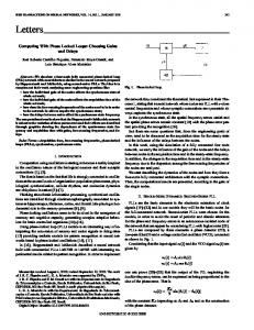
(2) with (2a) and (2b) where error performed over training set (“current” knowledge); corresponding error over training set (“former” knowledge); output of the retrained network, corresponding to input vector of the network consisting of weights ; output of the retrained network, corresponding to input vector to the network consisting of weights . would represent the output of the network, Similarly, consisting of weights , when accepting vector at its input. is identical When retraining the network for the first time, . Parameter is a weighting factor accounting for the to significance of the current training set compared to the former denotes the -norm. one and In most real-life image or video analysis applications, training is a priori unknown; consequently estimation of as set well as detection of the change of the environment should be automatically provided by the system. As a result, apart from the retraining algorithm, two additional modules are embedded in the proposed architecture; a “change detection” decision mechanism and a MAP training set estimation procedure. The main objectives of these modules are briefly described next. A block-diagram of the overall architecture is presented in Fig. 1. The initially trained neural-network classifier and the retrained one are also included in the figure. The initially trained network is assumed to provide a coarse approximation of the correct classification irrespectively of changes of the environment. Possible misclassifications provided by this classifier are then corrected

DOULAMIS et al.: ON-LINE RETRAINABLE NEURAL NETWORKS

Fig. 1.

139

The system architecture.

by the retrained network, which generates the final classification. 1) Decision Mechanism: The goal of this module is to determine when retraining should be activated, or equivalently, to detect the time instances when a change of the environment occurs. Whenever network performance is considered satisfactory (no change of the environment occurs), the network weights and structure remain the same. Instead, new network weights are calculated when network performance is not appropriate, by activating both the MAP estimation procedure and the retraining algorithm. Investigation of the performance of the initially trained network on the current data is the basis of the mechanism, as described in Section V. 2) MAP Estimation Procedure: This module optimally selects a training set of input and desired output data which optimally represent the current situation as described in Section IV. This set is used next by the retraining algorithm described in the following section. III. THE RETRAINING TECHNIQUE

after retraining has been performed to a specific image or video frame. Let denote a vector containing the weights between the output and hidden neurons and , denote the vector of weights between the th hidden neuron and the network inputs, where subscripts refer to either the situation “after” or “before” retraining, and is respectively. An illustration of weights presented in Fig. 2. Then (3) is a vector containing all network weights. For a given input vector , corresponding to the th image block, the output of the final neural-network classifier is given by (4) denotes the activation function of the output neuron, where e.g., a sigmoidal function, and

A. The Network Architecture Let us, for simplicity, consider: 1) a two-class classification refer, for example, to foreground problem, where classes , and background objects in an image and 2) a feedforward neural-network classifier which includes a single output neuron providing classification in two categories, one hidden layer consisting of neurons, and accepts image blocks of, say, pixels at its input. Let us also ignore neuron thresholds. Extension to classification problems and networks of higher complexity can be performed in a similar way. Fig. 2 presents and the structure of the network. As mentioned before, denote the corresponding network weights, before and

(5) is a vector containing the hidden neuron outputs when the net(before retraining) or (after the rework weights are training). The network output in (4) is scalar, since we have assumed a single network output. The output of the th neuron of the first hidden layer can be written in terms of the input vector as follows: and the weights (6)

140

Fig. 2.


The neural-network structure.

Thus (5) can be expressed as (7)

network knowledge. To stress, however, the importance of current training data in (2), one can replace (2a) by the constraint that the actual network outputs are equal to the desired ones, that is for all data in

where matrix defined as vector-valued function the elements of which represent the activation function of a corresponding hidden neuron. The hyperbolic tangent sigmoidal function is used in the rest of the paper.

(9)

Equation (9) indicates that the first term of (2), corresponding to , takes values close to zero, after estimating the new error network weights. It is shown in Appendix B that, through linearization, solution of (9) with respect to the weight increments is equivalent to a set of linear equations

B. The Retraining Algorithm

(10)

The goal of the training procedure is to minimize (2) and esand , respectimate the new network weights , i.e., tively. Let us first assume that a small perturbation of the netis enough to achieve good work weights (before retraining) classification performance. Then and

(8)

and are small increments. This assumption where , leads to an analytical and tractable solution for estimating since it permits linearization of the nonlinear activation function of the neuron, using a first-order Taylor series expansion. Equation (2) indicates that the new network weights are estimated taking into account both the current and the previous

, , with denoting a vector formed by stacking up all columns ; vector and matrix are appropriately expressed in of is terms of the previous network weights. The size of for the network presented in Fig. 2. In particular, , expressing the difference between network outputs after and before retraining for all input vectors in . Based on (9), vector can be written as

where

(11) are Equation (10) is valid only when weight increments small quantities. In Appendix A, (A11) and (A13), it is shown


141

that, given a tolerated error value, proper bounds and can be computed for the weight increments, for each input vector in

and (12) where is a vector depending on the former weights and on the input vector as described in Appendix B. Equation (12) should be satisfied for all in , so as to assure that each linear equation in (10) is valid within the given tolerated error. A less strict approach would require that the mean value of the inner products in (12), for all , be smaller than the mean value of the bounds. The size of vector is smaller than the number of unknown , since in general a small number, , of training weights data, is chosen, either through a clustering or a principal component analysis technique. Thus, many solutions exist for (10), since the number of unknowns is much greater than the respective number of equations. Uniqueness, however, is imposed by an additional requirement, which takes into consideration the previous network knowledge. Among all possible solutions that satisfy (10) the one which causes a minimal degradation of the previous network knowledge is selected as the most appropriate. It is considered that the network weights before retraining, i.e., , have been estimated as an optimal solution over data of set . Furthermore, the weights after retraining provide a minimal error over all data of the current set , according to (9). Thus, minimization of the second term of (2), which expresses the effect of the new network weights over data set , can be considered as minimization of the absolute difference of the error over with respect to the previous and the current network data in weights. Similar conclusions are drawn in [31]. This means that the weight increments are minimally modified, resulting in the following error criterion: (13) defined similarly to , with replaced by with the right-hand side of (2b). It can be shown [31] that (13) takes the form of

in

(14) are expressed in terms of where the elements of matrix and the training data in . the previous network weights Thus, the problem results in minimization of (14) subject to constraints (10) and (12). is in general much The number of data belonging to set smaller than the number of network weights. This is due to the fact that these data have been selected from the current condition using a clustering or principal component analysis technique to discard data of similar content and obtain more reliable solutions. Thus, network overfitting could arise if only these current data were taken into account. However, in our method, the network weights are estimated using data from both the current set and the previous set , as (10) and (14) indicate. The number

of elements of is in general greater than the number of network weights since this set includes all a priori network knowledge. Consequently, overfitting issues are not encountered in the proposed retraining algorithm, since the number of training and , is greater than the data, i.e., the number of data in respective network weights. In Section V, where experimental results are presented, specific values for the numbers of data in and are provided. sets The error function defined by (14) is convex since it is of squared form [25]. The constraints in (10) are linear equalities, while the constraints in (12) are linear inequalities. Thus, the solution should lie on the hyper-surface defined by (10), satisfy the inequalities in (12) and simultaneously minimize the error function given in (14). A variety of methods can be used to estimate the weight increments based on minimization of (14) subject to (10) and (12). In this paper we adopt the gradient projection method, which is presented next. As described in Section V, the decision mechanism ascertains whether a small adaptation of the network weights is sufficient to provide accurate classification. In case that such a small adaptation is not adequate, the above training algorithm cannot be used, since the activation functions cannot be approximated by a first-order Taylor series. In this case, neither (9) nor (13) can be expressed in a simple form and thus the new network weights should be estimated through conventional minimization of (2) by applying, for example, the backpropagation algorithm. Since both the current and previous network training data sets are taken into account for updating the weights, overfitting issues are not encountered in this case too. Each time the decision mechanism ascertains that retraining is created, which represents is required, a new training set the current condition. Then, new network weights are estimated taking into account both the current information (data in ) and the former knowledge (data in ). Since the set has been optimized over the current condition, it cannot be considered suitable for following or future states of the environment. This is due to the fact that data obtained from future states of the environment may be in conflict with data obtained from the current one. On the contrary, it is assumed that the training set , which is in general provided by a vendor, is able to roughly approximate the desired network performance at any state of the environment. Consequently, in every network retraining phase, a new training set is created and the previous one is discarded, while new weights are estimated based on the current set and the old one , which remains constant throughout network operation. C. The Gradient Projection Method The philosophy of the gradient projection method is, starting from a feasible point, to move in a direction which decreases and simultaneously satisfies the constraints (10) and (12). Let us give some definitions first [25]. A point is called feasible when it satisfies all the constraints. An inequality is characterized as an active constraint when it is about to be violated at a feasible point, in the sense that it turns to equality at this point. Otherwise the inequality is an inactive constraint. For example, in (12) becomes active at the inequality when at this current a feasible point

142


point. Otherwise it is considered to be inactive. In the following the number of active inequalities. By convenwe denote as tion we consider any equality constraint to be active at a feasible point. Thus, the total number of active constraints, i.e., equali( equalities ties and active inequalities, is equal to active inequalities). and Only the active constraints define the direction which causes . As a result, a working set is formed at a decrease of function each feasible point which includes all active constraints. Then, the method tries to move in a direction which decreases the error while keeping the working constraints active. This function onto is accomplished by projecting the negative gradient of the subspace that is tangent to the surface defined by these constraints. If the resulting vector is nonzero, it determines the direction for the next step. To compute this projection, let matrix be composed of the above-defined working set. Matrix contains all rows of matrix (since equalities are always active at any feasible point) and additional rows which include the acis of , where we recall tive inequalities. Thus, corresponds to the total number of network weights. Let that the projection of the negative gradient of us denote by in the th iteration step of the algorithm. Then, adaptation of the weight increments is made as follows:

the obtained solution. It should be mentioned that the times that the working set is changed are equal to number of inequalities since equalities are always considered active. Thus, the number of iterations required for getting all elements of positive so that the Kuhn–Tucker conditions are satisfied, is bounded by the number of inequalities. The time required to adapt network weights is very crucial, especially in real-time applications. This is, for example, the case in video processing, where each video frame is transmitted every 40 (33) ms for the PAL (NTSC) system and thus network retraining should be completed within this small interframe period. The computational complexity required to update each network weight independently using the gradient projection method is proportional to the number of network weights as shown next. At each iteration of the algorithm, the inner product of mais calculated (16a) along trix with the gradient of function is of with the weight updating given by (15). Since function and thus (16a) squared form, the gradient with matrix involves a simple multiplication of vector , which is of size . This requires operations assuming that each element of can be implemented in parallel. It should be mentioned that matrix , for a fixed number of working constraints is calculated once since is modified each time the working constraints are changed and matrix , which depends on the previous network weights , is available before the algorithm begins. Furthermore, the projection matrix does not need to be entirely recomputed each time the working constraints are modified. This is due to the fact that the active constraints in the working set change by one at a time and thus it is possible to recalculate matrix from the previous one by an updating procedure as described in [25, p. 333]. This is a significant property of the gradient projection method and greatly reduces its computational load. The convergence rate of the gradient projection method is of the same order with that of steepest descent, for a constant ; i.e., it converges to the optimal solution linlearning rate early as can be shown using eigenvalue analysis in [25, p. 342]. Faster convergence rates can be achieved by selecting the value to be the largest step toward the global minimum. This can be accomplished by minimizing the following equation with re: spect to learning rate

(15) is a scalar that determines the rate of convergence. where as Using the methodology of [25] we can estimate vector (16a) with and

(16b)

computed from (14) at the th iteration. using Starting from an initial feasible point, the gradient projection algorithm computes the next feasible point based on (15) until is close to zero, i.e., . In the projected gradient this case, however, it is possible to improve the solution (esti) mate a new feasible point that causes a greater decrease of by relaxing one active constraint, i.e., one active inequality. This happens since the Kuhn–Tucker conditions are not satisfied for the original problem [25]. A vector, say , is calculated by the following equation: (17) Each element of , denoted as , corresponds to the th active constraint of the working set [25]. In case that there are negative elements of , the Kuhn–Tucker conditions are not satisfied and a new improved feasible solution can be obtained by relaxing the respective constraint from the working set. This is performed by deleting the corresponding row of , so that the respective constraint becomes inactive. In this case the projechas modtion matrix should be recomputed since matrix ified. A new iteration then commences until the projected grareaches a value close to zero. If all elements of are dient nonnegative, the Kuhn–Tucker conditions are satisfied and the process is terminated since it is not possible to further improve

(18)

After minimization, the optimal value of learning rate the following:

is

(19)

The number of iterations required by the algorithm to converge is further restricted by the maximum permitted time, say , in which retraining should be accomplished. For instance,


143

in case of on line classification of video frames, ms for a PAL system, within which selection of the current training set , weight adaptation procedure as well as network testing using the new weights should be completed. Since the time required for network retraining is significantly larger than the other times, we can assume in the following that the maximum permitted time for weight adaptation is approximately . Thus, the number of iterations of the gradient proequal to , where indijection method should be smaller than cates the average computational time for one iteration. If, after iterations, the solution is not close to the optimal one, the currently estimated weights are used to perform classification. Weight updating will be continued in the following frames, for further improving the network performance. Similarly, in a large weight adaptation case, where a type of backpropagation algorithm is used for estimating the network weights, the number of . iterations is also restricted by the maximum permitted time , processing moves to If a solution cannot be reached within the following frames, assuming that no further retraining is required.

It is straightforward to show that the corresponding conditional probability density can be written as follows:

(22) where we have ignored the dependence on the current image , since it is involved in all equations. Estimation of the network weights is independent of vector . Moreover, network output only depends on the values of the weights (and the input image). Hence, it can be concluded that

(23) Using (4), (5), and (7), it is easy to compute a nonlinear functhat models the operation of the neural network. Then tion (24)

IV. OPTIMAL SELECTION OF THE NETWORK RETRAINING DATA Whenever the decision mechanism ascertains that network retraining is required, a training set should be generated so that the retraining algorithm uses it to adapt the network weights to the current environment. A MAP estimation procedure is proposed next for constructing this training set , i.e., for de, with denoting input image termining proper pairs blocks of the examined image and respective desired outputs. Let be a vector containing the probabilities that each image block belongs to one of the available classes. Then, where is the number of . A high value blocks of image and indicates that it is highly probable that the respective image block belongs to class and can therefore be included in the retraining set, being classified to category . Let also vectors and include the outputs of the retrained and initially trained networks, respectively, for all blocks of image , i.e.,

and (20) For a current image and an output being provided by the initially trained network, our target is: 1) to estimate vector , and consequently the current training set ; 2) to compute the (through the retraining weights of the final network classifier algorithm); and 3) to obtain the final classification output corresponding to image . This can be obtained through maximization of the following conditional likelihood function:

Thus, if the optimal weights have been estimated through network retraining, the final classification of current image is unique. Consequently if fullfils (24) otherwise.

(25)

Equation (23) using (25) indicates that the optimal vector and the output of the retrained classifier can be computed as follows:

(26) Optimal network weights are calculated by the retraining algorithm of Section III given a vector , i.e., the training set . Thus, maximization of the latter term in (26) is achieved through by the retraining algorithm. Consecomputation of weights quently, maximization of (26) is equivalent to estimation of (and consequently ), based on the output of the initially trained neural classifier. Thus (26) results in (27) Using the Bayes formula, (27) can be written as follows:

(21)

(28)

where denotes a log-likelihood function. In (21) denotes the provided by the retraining algorithm and is the weights classification output of the retrained neural-network classifier which is applied to the input image .

has been omitted from the log likelihood function, where since it is independent of . Equation (28) indicates that in order to find , we should compute both the conditional probability and the probability density . density

144


Let us first assume that for a given vector , there is only one classification vector which is associated to by a linear relation through a fixed matrix , or equivalently that different training sets are estimated for different vectors . As a result, is given by the conditional probability density

choice for function in a two-class classification problem, is a scalar denoted by , is where

if if

(29)

. The elThe next step is to model probability density ements of represent the probabilities that an image block belongs to each of the available classes. It is well known that are strongly correlated to their spatial neighimage blocks bors, due to smoothness of the objects appearing in images. are also locally correlated, i.e., for Thus, the elements of we have [5], [20] image blocks and

(30) denotes a neighborhood of the image block correwhere sponding to . Such a property characterizes an MRF, hence [5], [15], a Gibbs distribution can be used for modeling [35]

(31)

where normalizing constant; “temperature” parameter of the density; any function of a local group of points called clique and is the set of all cliques. Using the MAP estimation procedure and based on (28) and (29) the estimate of can be written as (32) Based on the previous equation, it is observed that estimation of the optimal vector is not affected by the value of temperature since the latter has the same influence on all directions of the clique. For this reason, we will consider, for simplicity, in . the following that As already mentioned, images are locally smooth [38]. Consequently, it is not probable that an image block belongs to a specific class, if all its neighbors belong to another one. Since retraining should be performed using data that have already been classified with maximum confidence, function should award image blocks that satisfy the smoothness property and discourage the rest. It should also be mentioned that the knowledge included in the initially trained network classifier should be trusted as much as possible within the above selection procedure; it is, therefore, desired that the finally computed classification is similar to the one originally provided by the classifier, modified according to the smoothness principle. Following the previous assumption, a common

(33a) where measure depends both on the distance of from the corresponding initial classification as well as on its distance from its neighbors . In (33a), the neighborhood of , i.e., the clique structure, has been selected to be a 3 × 3 pixel grid. An equal-weight operator has been used for all eight directions of the clique, since the same training set should be produced irrespectively from the image orientation. For this reason, function in (33a) is given by (33b) where parameter controls the contribution of each of the two terms in the right-hand side of (33b) to the minimization of the cost function. In particular, values of close to zero result in a vector that approximately equals output obtained by the initially trained classifier. However, several misclassified blocks as was mentioned in Section II. Since are encountered in training set , which is used for network retraining, follows the estimation of the optimal vector , erroneous training elefor small values of . As a rements will be presented in sult, the network performance deteriorates after retraining. On the other hand, unnecessarily large values of stress the importance of the smoothness (second) term of (33b), resulting in many ambiguous blocks, i.e., blocks which do not present high probability of belonging to a specific class. In this case the set cannot appropriately describe the current condition since it contains few training data, i.e., only those which are not ambiguous. As parameter increases from small to large values, more are considered as amand more misclassified blocks of biguous and are therefore discarded from . However, very large values of reduce the representativity of , since high confident blocks are also discarded apart from the misclassified contains % misclassified ones. Assuming that the output is selected so that the training set blocks, the parameter contains a slightly smaller number than 1- % of the total number of image blocks; a slight deviation of around the selected value does not significantly affect network performance after retraining. in (33b) satisfies the convexity property since it Function is of squared form [25]. Therefore, (33a) also defines a convex function since the sum of convex functions also yields a convex function (see [25, p. 178, Proposition 1]). Convexity guarantees that a global minimum can be obtained by minimizing (32). Otherwise, local minima would be present and a computationally expensive technique, such as simulated annealing [24], should be used for function minimization. Direct minimization of (32) leads to the linear relation between and that has been assumed in (29). In (33a) and (33b) the value of depends on the values of the eight connected neighbors (located on the clique structure), which are also involved in the minimization process. For this reason, the iterative conditional modes (ICM’s) technique [3] has been proposed to estimate the optimal vector .


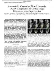
Fig. 3.

145

A scenario of a video sequence consisting of eight frames in which retraining at frames three and six has been accomplished.

Starting from an initial, say zero, condition, the algorithm converges in a few steps to the minimum value of . Following computation of optimal vector , selection of the for retraining the classifier can be performed as foldata set lows. Let us denote by a set of indexes , which correspond to elements of vector , say, , which belong with high probability to one of the two classes (34) and are proper thresholds which define the regions where of high probability. If we denote by the th element of set , are included in . then the pairs Although in general the above described method converges to the optimal value after a small number of iterations, in case of real-time applications, where the amount of computational cost is very crucial, alternative techniques can be used for selection of the training set . A fast technique, which yields a suboptimal but good selection of training data, is based on the binary form of the mask of the initially trained network. This form is derived by thresholding the probability values of (1) for all image blocks. Then, a block is selected as training one, if all its eight neighbors belong to the same class with it. In this way, ambiguous blocks are discarded from the training set and only the most confident ones are selected for training, through a very fast procedure. V. THE DECISION MECHANISM FOR NETWORK RETRAINING The purpose of this mechanism is to detect when the output of the neural-network classifier is not appropriate and consequently to activate the retraining algorithm at those time instances when a change of the environment occurs. Let us index images or video frames in time, denoting by the th image or image frame following the image is at which the th network retraining occurred. Index therefore reset each time retraining takes place, with corresponding to the image where the th retraining of the network was accomplished. Fig. 3 indicates a scenario with two retraining phases (at frames three and six, respectively, of a video sequence composed of eight frames) and the corresponding values of indexes and . It can been seen that where indicates that after

images from the th retraining phase, a new retraining phase, th takes place. i.e., the Retraining of the network classifier is accomplished at time instances where its performance deteriorates, i.e., the current network output deviates from the desired one. Let us recall that vector in (11) expresses the difference between the desired and apand the actual network outputs based on weights plied to the current data set . As a result, if the norm of vector increases, network performance deviates from the desired one and retraining should be applied. On the contrary, if vector takes small values, then no retraining is required. In the folindicating its depenlowing we denote this vector as . However, direct calculation of the dence upon image would require application of the MAP estinorm of mation procedure described in the previous section so as to exfrom each image . In video processing applitract cations, for example, each image frame arrives at a rate of 40 ms (25 frames/s in PAL system); it will therefore be very time consuming to activate the MAP estimation procedure for each . In such applications, detection of the retraining time instances can be performed through the following methodology. A. Detection of the Retraining Time Instances Let us assume that the th retraining phase of the network classifier has been completed. If the classifier is then applied to , including the ones used for reall blocks of the image training, it is expected to provide classification results of good quality. The difference between the output of the retrained network and of that produced by the initially trained classifier at constitutes an estimate of the level of improveimage ment that can be achieved by the retraining procedure. Let us this difference, which is computed as foldenote by lows:

(35) where is the number of blocks in the image; dependence of vector on the current network weights has been omitted for simplicity. denote the difference between the corresponding Let classification outputs, when the two networks are applied to the

146


th image or image frame following the phase, for

th network retraining

(36) It is anticipated that the level of improvement expressed by will be close to that of as long as the classification results are good. This will occur when input images are similar, or belong to the same scene with the ones used during , which is quite different the retraining phase. An error , is generally due to a change of the environment. from can be used Thus, the quantity for detecting the change of the environment or equivalently the time instances where retraining should occur. Thus if

no retraining is needed

(37)

where is a threshold which expresses the maximum tolerance, beyond which retraining is required for improving the network performance. In case of retraining, index is reset to zero while index is incremented by one. Such an approach detects with high accuracy the retraining time instances both in cases of abrupt and gradual changes of the operational environment since the comparison is performed and the one obbetween the current error difference . In an abrupt operatained right after retraining, i.e., will not be close to ; contional change, error exceeds threshold and retraining is actisequently, will graduvated. In case of a gradual change, error so that the quantity gradally deviate from ually increases and retraining is activated at the frame where . in (11) is not directly involved The norm of vector in (37). Since in (36) corresponds to in (11) and ’s are replaced by ’s, it can be concluded that, (36) uses the output provided by the initially trained network as an approximation of the desired output in each new image, or frame. For detection purand the norm of appear to have similar poses provides a quick way behavior and properties and thus for determining the retraining time instances without requiring to activate the MAP estimation procedure at every image frame . Network retraining can be instantaneously executed each time the system is put in operation by the user by utilizing zero initial values for the output mask . Thus, the quantity initially exceeds threshold and retraining is forced to take place. In some, rather rare, cases, the aforementioned mechanism could detect no need for retraining although it should. This is, for example, the case when a significant amount of image blocks lie near class boundaries, and consequently there is low probability that they belong to a specific class. Thus, despite a possible large change in the classification of the image blocks, due to moving boundaries, there is only a small variation of the block probabilities. In this case, the decision mechanism detects no need for retraining since only a small perturbation of the block probabilities has occurred. To avoid such situations, the binary and can be used in (35) and (36) as an forms of masks

additional or alternative mechanism for detecting the need for retraining. This is due to the fact that masks and , in binary form, suffer large variation for any change of the environment; and thus, they cause a large variation of the difference as a consequence, retraining is activated. Other measures that can be also used for detecting the need of retraining are the comparison of the spatial distribution of classified blocks to that of each class as well as of their number with respect to total number of blocks in the image. B. The Retraining Phase exceeds threshold for some , say , the th retraining phase starts. In this case, the MAP estimation procedure is activated so as to create the training set which represents the current condition; vector is also calculated. The weights of the network bein the fore retraining are used as previous network weights retraining algorithm. The training algorithm provides the new network weights through minimization of (14) subject to constraints (10) and (12). However, existence of a feasible solution is assured only if the hyper plane given by (10) crosses through the boundary constraints imposed by (12). For this reason the minimal distance , is from the origin to the surface first calculated, by solving the following minimization problem with respect to When

minimize or equivalently subject to (38) Using Lagrange multipliers the above minimization problem leads to the following solution: with (39) is the minimal distance from the origin to . For this value of , if the inequality constraints defined by (12) are satisfied for all data in , the new network weights can be calculated by minimizing (14) subject to (10) and (12). Otherwise, (2) cannot be expressed in the simple form of (10) and (14) and thus direct minimization of (2) is required for estimating the network weights. This is due to the fact that the former knowledge is quite different from the current one and a small weight perturbation is inadequate for sufficiently adapting the network weights. Another situation where the above can be used is the following. Let us assume that several neural-network classifiers along with their respective training sets and weights have been given to a user by different suppliers or that the user has created different retraining sets himself using the procedure presented in the paper; the user is assumed to apply one of them. In cases that the decision mechanism detects that retraining is needed, but the training algorithm cannot be applied to the users’ classification problem since the boundary constraints are not satisfied, it seeks, among the available networks, the most appro-

where


147

TABLE I

TABLE II

TABLE III

priate one for the current environment. Then, the selected network is considered to represent the best previous knowledge and the training algorithm is used to further improve the network performance. The inner steps of the method, i.e., the retraining algorithm, the selection of retraining data and the decision mechanism are given in algorithmic form in Tables I–III of this paper. VI. EXPERIMENTAL STUDY In the following, the performance of the proposed scheme for on line neural network retraining was examined for detection

and extraction of humans, and particularly of the upper part of human body including the head, shoulders and arms areas, in images or video sequences. Such an extraction plays an important role in many image analysis problems. Examples include retrieval of images or video sequences containing humans from image data bases [9], [11], [13] low bit rate coding of image sequences for videophone and videoconferencing applications [8], [10], [36], video surveillance of specific areas, such as city centers, for identifying suspects for crimes [14], as well as analysis by synthesis methods, where 2-D or 3-D modeling follows the extraction of human bodies from scenes. Furthermore, human extraction from background has recently attracted a great

148

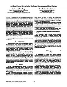
Fig. 4. The error-fuction a(k; N ) computed by the decision mechanism (solid line) along with the threshold T beyond of which retraining is required (dashed line). For comparison the kc(k; N )k is also shown in the figure.

research interest especially in the framework of MPEG-4 and MPEG-7 standards for content-based video coding/representation and content-based visual query in image and video. An image scene was formed consisting of 40 frames from three different color videophone sequences, Claire, Trevor, and Miss America. In particular the sequence consisted of ten frames of Claire, followed by ten frames of Claire with their luminosity changed, followed by ten frames of Trevor and by ten frames of Miss America. Thus, the image scene included three changes of the environment. Several characteristic data of video conference applications has been used to train the initial neural-network classifier. The format of the three-color sequences was QCIF, i.e., each image frame consisted of 144 × 176 pixels per color image component. The latter were separated in image blocks consisting of 8 × 8 pixels, resulting in = 396 blocks per component. The target was to classify each image block into one of two classes, namely foreground objects, i.e., upper part of human body, and background. The dc coefficient and the first 8 ac coefficients of the zig-zag scanned DCT transform of each color component of the th block, i.e., 27 elements in total were used as input to the network, which consisted of = 15 units in the hidden layer and one output unit as described in Section III-A. This results in 450 network weights, apart from the biases. The set contains approximately 1000 image blocks as training elements. , computed by the proposed decision Fig. 4 shows, estimated mechanism using (35), (36), and the norm of by applying the MAP procedure to each image frame. For clarity by of presentation we have multiplied the values of the factor of five. Similar behavior of the value of and is observed. It can be seen that using a constant threshold of 4% the proposed mechanism was able to correctly detect whether retraining was required or not. After network initialization, where retraining has been activated on the first was below the value of 4% in the frame of Claire, the following frames and therefore no retraining was needed. On the other hand, at the first frame of the Claire sequence with a exceeded the threshold luminosity change, the value of and the decision mechanism activated the retraining algorithm


for adapting the network weights to the current condition. The same happened at the first frames of Trevor and Miss America. The retraining algorithm, described in Section III, was used to adapt the network weights in all the above changes of the scene. Fig. 5 shows the values of the 27 network weights connecting 1) the first hidden and 2) the tenth hidden neuron to the network input computed in the case of Claire before and after the luminosity change. The procedure described in Section IV was used for optimally selecting the retraining data sets and providing them to the training algorithm. In all the above cases the inequality constraints imposed by (12) were satisfied. The relative tolerance error of the network output was chosen to be less than 10%. Since, the desired output for all training data in , corresponding to foreground (background), was close to 1 (−1), the bounds in (12) were almost equal, for all training inputs . For the selected relative error, was equal to 0.5, while was calculated based on (A7) and (A12) and was equal to 0.38 for the first frame of Claire sequence with luminosity change. Fig. 6 illustrates the inner product of (A13) for the weights connecting the first and the tenth hidden neurons to the input layer, for all input vectors in . The next figures refer to the quality of classification achieved by the proposed system. Fig. 7(a) shows a characteristic frame of the Claire sequence, while Fig. 7(b) the first frame of Claire with a luminosity change, where retraining was performed. Fig. 7(c) shows the classification output provided by the network after retraining (final classification). The output is shown in the form of a map, in which all blocks classified to belong to background are, for clarity of presentation, marked with black color. It is observed that, after retraining, the network correctly classifies the image blocks into the two categories. Fig. 7(d) illustrates the network output before retraining. It is clear that several blocks, mainly in Claire’s body, have been misclassified due to the luminosity change. The output of the MAP estimation procedure, which was used for selecting the retraining data set is presented in Fig. 7(e) in continuous form. In this case the parameter has set contains about 70% of the total been selected so that the . This is due to the number of image blocks; its value was fact that it is assumed that the initially trained network provides an approximation slightly greater than 70% for the final classification (30% misclassification). Dark blocks indicate areas of background, white blocks indicate foreground areas while gray ones indicate ambiguous areas. This mask has been generated by minimizing (33a) and (33b) with respect to vector . A 3 × 3 pixel grid with equal weights in all eight directions has been selected to form the clique structure, as was mentioned in Section IV. Fig. 7(f) also shows the selected training blocks, in discrete form; black color denotes all blocks that were not selected as training data. Since there is a large number of similar training blocks, especially in the background, a distance measure was used to reduce their number before using them to define the constraints in (10). The number of selected blocks was reduced, in this way, from 198 to ten. Fig. 8 refers to network retraining when fed with the first frame of the Trevor sequence, shown in Fig. 8(a). Fig. 8(b) shows the output of the initial network, which provided a coarse approximation of the desired classification. The effect of paramis illustrated in Fig. 9. In eter on selecting the training set


149

Fig. 5. Weight adaptation by the training algorithm in case of the Claire sequence with luminosity change. The weights between the input layer and (a) the first hidden neuron, i.e., w and (b) the tenth hidden neuron i.e., w .

Fig. 6. The inner product of network weight perturbation, corresponding to the weights connecting the input layer to (a) the first and (b) the tenth hidden neuron, respectively, for all input vectors of the training set S in case of Claire sequence with luminosity change (solid line). The bound derived from (A7) and (A12) is illustrated in dashed line.

this figure the selected foreground blocks are depicted for two extreme values of ; = 0.5, and = 22. As is observed, when is close to zero, erroneous training data are estimated. Instead, large values of result in a small training set, which is generally inadequate to represent with high accuracy the current image. Fig. 10 presents the percentage of the selected training to the total number of image blocks versus paramdata in eter . It can been seen that the number of selected blocks to that of the total image decreases as the value of increases. Having assumed that the initially trained neural network approximates the desired classification by about 70%, the parameter is selected so that the percentage of the selected data is 70% of the total blocks. Fig. 8(c) shows the output of the MAP estimation technique in a form similar to that of Fig. 7(e) using the value of selected from Fig. 10 ( = 4.92). Fig. 8(d) shows the training set selected by the MAP estimation procedure in this

case. Moreover, the convergence of the MAP estimation procedure is shown in Fig. 11, in terms of the number of blocks moved from one class to the other in consecutive iterations. It can be easily seen that, starting from a zero initial value of , the algorithm converges within five iterations to the global minimum of the cost function (33a) and (33b). Fig. 8(e) presents the network output after retraining, which shows that correct classification has been achieved. In the following, a video conference application showing a scene of a conference room with three people talking is examined. In this case, since the scene can be considered as superposition of three video frames, each of which presents a single person, the initially trained neural-network classifier will continue to provide satisfactory results. After network retraining, extraction of foreground objects from background is very satisfactorily accomplished. The first frame of the respective se-

150


Fig. 7. (a) A characteristic frame of Claire, (b) the first frame of Claire with luminosity change, (c) the classification output, in discrete form, after network retraining, (d) the network output before retraining, for the same frame, in discrete form, (e) the training set S selected for retraining, in continuous form, i.e., the output of the MAP estimation procedure, set S , and (f) in discrete form.

quence is depicted in Fig. 12(a). Fig. 12(b) shows the respective training set in binary form, while Fig. 12(c) the final classification results. As far as the problem of foreground–background separation is concerned, the proposed neural-network architecture provides very accurate results regardless of the luminosity conditions, foreground–background location/orientation and the respective

color characteristics as Figs. 7 and 8 indicate. Segmentation techniques based on spatial and/or texture homogeneity criteria have been also proposed in the literature for this purpose [6], [27], [34], [37]. However, such approaches cannot provide accurate foreground–background separation since, in general, a person in a scene, contains regions with different color and texture characteristics (e.g., head, hair, clothes’ color) which are


151

Fig. 8. Network performance at the first frame of Trevor sequence: (a) the original image, (b) the output of initially trained network, (c) the training set S selected for retraining in continuous form, (d) the training set in discrete form, and (e) the final classification output in discrete form.

classified to different segments (objects) according to such homogeneity criteria. For example, division of a square image into four equal-sized square blocks (quadtree decomposition), according to the texture homogeneity of the block, results in many misclassified blocks both in background and foreground areas [10]. Recently, other approaches have been proposed in the literature, which combine (fuse) several image properties according to predefined rules in order to provide more semantic video ob-

ject extraction [2], [26]. However, these methods are restricted to the specific applications and thus they cannot be applied to different operational conditions. VII. CONCLUSIONS This paper has discussed on-line retraining of neural networks, focusing on image and video analysis applications. A training al-

152


Fig. 9. The selected foreground blocks for different values of parameter : (a) = 0.5 and (b) = 22.0.

Fig. 10. .

Variation of the percentage of selected image blocks versus parameter

gorithm has been presented, which can efficiently handle cases of smallvariationsoftheoperationalenvironment,whileamaximum a posteriori estimation technique has been developed which optimallyselectstheretrainingdatasetfromtheimagepresentedtothe network. This is accomplished by modeling the image as an MRF. A decision mechanism has also been introduced which automatically activates network retraining whenever the network performance is not considered satisfactory. The presented results refer to extraction of foreground areas from background ones in image/video classification problems. These results indicate the ability of the method to be successfully applied to a variety of image analysis applications, where neural-network-based classification constitutes a possible solution, especially when considering the forthcoming MPEG standards. This constitutes a topic, which is currently further investigated. It should be mentioned that the proposed neural-network architecture can be used to a variety of other applications. Examples include prediction of video traffic over high-speed networks where the traffic characteristics vary from time to time according to the scene complexity or nonlinear system identification where the system to be identified is changing with time. As a result, the proposed scheme can be viewed as a method for

Fig. 11. Trevor.

Convergence of the MAP estimation procedure at the first frame of

improving the performance of neural networks in dynamically changed environments. Of particular interest is the interweaving of MAP estimation algorithms with neural-network learning optimization algorithms; in the resulting scheme optimal selection of the network training set is performed by the former algorithms and optimal output estimation is provided by the neural network. Investigation of convergence and performance of a general block component estimation method, which iteratively uses these two procedures, is another topic, which is under investigation. APPENDIX A , , As was described in Section III, network weights before and after retraining, respectively, are related through the following equation: (A1) denotes a small perturbation. where Using (6), the output of the th neuron of the hidden layer, after retraining, is given by (A2)


153

Fig. 12. Network performance for a video scene indicating a conference room with three people talking: (a) the original image, (b) the training set selected in discrete form, and (c) the final classification mask.

omitting, for simplicity, subscript on . pendence of From (A2) it can be seen that ; setting product form

from

as well as the de-

depends only on the inner , (A2) takes the

where second derivative of ; scalar taking values between and . in (A5) should be In general the absolute value of bounded, so that the error of the first-order Taylor series be small, i.e.,

(A3)

(A6)

Combining (A1) and (A3) and using the formula of first-order Taylor series expansion we have

is the maximum error of the residual , that is alwhere lowed. Based on (A6) and using the Lagrange formula (A5), the inner can be bounded as follows: product

(A4)

(A7)

is the output of the th hidden neuron before the rewhere with , training phase, i.e., is a small perturbation, , with and . Function in (A4) denotes the first , while represents the first-order Taylor derivative of residual for the th hidden neuron. Using the Lagrange formula, can be expressed as (A5)

in (A7) is difficult to be calculated, since The value of can be performed by scalar is unknown. Estimation of is bounded and considering that the second derivative of be equal to its maximum value, , by letting . From (A7) we get two linear inequalwhere so that the first-order Taylor series expansion be ities for valid with an error less than , namely

154


Using (4) and ignoring the residual errors in (A4), we can express the network output , after retraining, as follows:

where is the number of neurons in the first hidden layer. In this are the same, i.e., case all bounds of the inner product (A13) APPENDIX B

(A8) has been ignored since it is very small where the term compared to the other terms. Let us recall that , are vectors is defined as defined in (6), while . Expanding (A8) as a first-order Taylor series we get

and ignoring residual For a given input vector in (A9), we can approximate the network output as follows:

in (B1)

where we have introduced the dependence of the output on input vector . Using (9), (B1) is written as (B2) [see (A8)] Since indicating a linear relationship with the total weight perturbation , the term in (B2) can be expressed as

(A9) and . In (A9), represents the residual error of the first-order Taylor series approximation which can be expressed similarly to (A5). Requiring that the residual is , smaller than a relative error provided by the user, say, the following inequality should be satisfied: where we have set

(B3) where equation:

is a vector provided by the solution of the following

(B4) Since

depends on the network weights, we have (B5)

(A10) with is known, being It should be mentioned that the value of estimated by the MAP estimation procedure. can be performed similarly to (A7). As Computation of can be written as , is proved in Appendix B, where is a vector depending on the weights before retraining and on the input vector . Consequently (A10) imposes two is linear inequalities as far as the total weight perturbation concerned

and The

the gradient matrix of the vector valued function is thus calculated by

.

(B6) (A11) Satisfaction of (A10) indicates that the approximate network output, using the first-order Taylor series expansion, differs , under the assumption from the actual one at most by . However, taking into consideration the that in (A4) the total error of the network output residuals . Let us denote is greater by an amount depending on of the first-layer by a vector containing all residuals . Then, using the mean neurons, i.e., value theorem, the error of the network output should be where . increased by the quantity and is a very small quantity, the Since previous term can be considered to be approximately equal . Using the Cauchy–Schwartz formula and to , the output error due requiring that is smaller than . Assuming for simplicity to residuals in (A6) are equal to each other, i.e., that all bounds of for all , we can estimate the residual bounds as (A12)

Taking into account all input vectors pressed as

in

, (B3) is ex(B7)

where and

REFERENCES [1] A. K. Aizawa and T. Huang, “Model-based image coding: Advanced video coding techniques for very low bitrate applications,” Proc. IEEE, vol. 83, pp. 259–271, 1995. [2] A. Alatan, L. Onural, M. Wollborn, R. Mech, E. Tuncel, and T. Sikora, “Image sequence analysis for emerging interactive multimedia services—The European cost 211 framework,” IEEE Trans. Circuits Systems Video Technol., vol. 8, no. 7, pp. 802–813, Nov. 1998. [3] J. E. Besag, “On the statistical analysis of dirty pictures,” J. Roy. Statist. Soc., ser. B, vol. 48, pp. 259–302, 1986. [4] A. Blumer, A. Ehrenfeucht, D. Haussler, and M. Warmuth, “Learnability and the Vapnik–Chervornenkis dimension,” J. Assoc. Computing Machinery, vol. 36, pp. 929–965, 1989.


[5] C. Bouman and K. Sauer, “A generalized Gaussian image model for edge-preserving MAP estimation,” IEEE Trans. Image Processing, vol. 2, pp. 296–310, 1993. [6] C. Bouman and M. Shapiro, “A multiscale random field model for Bayesian image segmentation,” IEEE Trans. Image Processing, vol. 3, no. 2, pp. 162–177, Mar. 1994. [7] B. Cheng and D. M. Titterington, “Neural networks: A review from a statistical perspective,” Statist. Sci., vol. 9, pp. 2–54, 1994. [8] L. Chiariglione, “MPEG and multimedia communications,” IEEE Trans. Circuits Syst. Video Technol., vol. 7, pp. 5–18, 1997. [9] A. D. Doulamis, Y. S. Avrithis, N. D. Doulamis, and S. Kollias, “Indexing and retrieval of the most characteristic frames/scenes in video databases,” in Proc. Wkshp. Image Anal. Multimedia Interactive Services (WIAMIS), Louvain-la Neuve, Belgium, June 1997, pp. 105–110. [10] N. Doulamis, A. Doulamis, D. Kalogeras, and S. Kollias, “Low bit rate coding of image sequences using adaptive regions of interest,” IEEE Trans. Circuits Syst. Video Technol., vol. 8, no. 8, pp. 928–934, Dec. 1998. [11] N. Doulamis, A. Doulamis, Y. Avrithis, and S. Kollias, “Video content representation using optimal extraction of frames and scenes,” in Proc. IEEE Int. Conf. Image Processing, Chicago, IL, Oct. 1998. [12] A. Eleftheriadis and A. Jacquin, “Automatic face location for model-assisted rate control in H.261 compatible coding of video,” Signal Processing Image Commun., vol. 7, pp. 435–455, 1995. [13] M. Flickner, H. Sawhney, W. Niblack, J. Ashley, Q. Huang, B. Dom, M. Gorkani, J. Hafner, D. Lee, D. Petkovic, D. Steele, and P. Yanker, “Query by image and video content: The QBIC system,” IEEE Comput. Mag., pp. 23–32, Sept. 1995. [14] J. Freer, B. Beggs, and H. Fernandez-Canqus, “Moving object surveillance and analysis of camera-based security systems,” in Proc. IEEE 29th Annu. Int. Carnghan Conf. Security Technol., U.K., 1995, pp. 67–71. [15] S. Geman and D. Geman, “Stochastic relaxation, Gibbs distributions, and the Bayesian restoration of images,” IEEE Trans. Pattern Anal. Machine Intell., vol. PAMI-6, pp. 721–741, 1984. [16] S. Haykin, Neural Networks: A Comprehensive Foundation. New York: Macmillan, 1994. [17] “Coding of moving pictures and associated audio for digital storage media at up to about 1.5 Mbps,”, ISO/CD 11172-2, Mar. 1991. [18] “Generic coding of moving pictures and associated audio,”, ISO/IEC 13 818-2, Recommendation H.262, Committee Draft, May 1994. [19] “MPEG-7: Context and objectives (v.3),”, ISO/IEC JTC1/SC29/WG11 N1678, Apr. 1997. [20] R. Kinderman and J. L. Snell, Markov Random Fields and their Applications. Providence, RI: Amer. Math. Soc., 1980. [21] S. Kollias, “An hierarchical multiresolution approach to invariant image recornition,” Neurocomputing, vol. 12, pp. 35–57, 1996. [22] S. Kung, “Neural networks for intelligent multimedia processing,” IEEE Signal Processing Mag., vol. 14, no. 4, July 1997. [23] T.-Y. Kwok and D.-Y. Yeung, “Constructive algorithms for structure learning in feedforward neural networks for regression problems,” IEEE Trans. Neural Networks, vol. 8, pp. 630–645, 1997. [24] S. Lakshmanan and H. Derin, “Simultaneous parameter estimation and segmentation of Gibbs random fields using simulated annealing,” IEEE Trans. Pattern Anal. Machine Intell., vol. 11, pp. 799–813, 1989. [25] D. J. Luenberger, Linear and Nonlinear Programming. Reading, MA: Addison-Wesley, 1984. [26] R. Mech and M. Wollborn, “A noise robust method for 2D shape estimation of moving objects in video sequences considering a moving camera,” in Proc. Wkshp. Image Anal. Multimedia Interactive Services (WIAMIS), Louvain-la-Neuve, Belgium, 1997. [27] F. Meyer and S. Beucher, “Morphological segmentation,” J. Visual Commun. Image Representation, vol. 1, no. 1, pp. 21–46, Sept. 1990. [28] MPEG Video Group, “MPEG-4 video verification model-version 2.1,”, ISO/IEC/JTCI//SC29/WG11, May 1996. [29] P. Mulroy, “Video content extraction: Review of current automatic algorithms,” in Proc. Wkshp. Image Anal. Multimedia Interactive Services (WIAMIS), Louvain-la Neuve, Belgium, June 1997, pp. 45–50. [30] N. G. Panagiotidis, D. Kalogeras, S. D. Kollias, and A. Stafylopatis, “Neural network-assisted effective lossy compression of medical images,” Proc. IEEE, vol. 84, pp. 1474–1487, 1996. [31] D. C. Park, M. A. EL-Sharkawi, and R. J. Marks II, “An adaptively trained neural network,” IEEE Trans. Neural Networks, vol. 2, pp. 334–345, 1991. [32] R. Reed, “Pruning algorithms—A survey,” IEEE Trans. Neural Networks, vol. 4, pp. 740–747, 1993.

155

[33] V. Ruiz de Angulo and C. Torras, “On-line learning with minimal degradation in feedforward networks,” IEEE Trans. Neural Networks, vol. 6, pp. 657–668, 1995. [34] P. Salembier and M. Pardas, “Hierarchical morphological segmentation for image sequence coding,” IEEE Trans. Image Processing, vol. 3, no. 5, pp. 639–651, Sept. 1994. [35] R. R. Shultz and R. L. Stevenson, “A Bayesian approach to image expansion for improved definition,” IEEE Trans. Image Processing, vol. 3, pp. 233–242, 1994. [36] T. Sikora, “The MPEG-4 video standard verification model,” IEEE Trans. Circuits Syst. Video Technol., vol. 7, no. 1, pp. 19–31, Feb. 1997. [37] C. Stiller, “Object-based estimation of dense motion fields,” IEEE Trans. Image Processing, vol. 6, no. 2, pp. 234–250, Feb. 1997. [38] A. M. Tekalp, Digital Video Processing. Englewood Cliffs, NJ: Prentice-Hall, 1995. [39] N. Tsapatsoulis, N. Doulamis, A. Doulamis, and S. Kollias, “Face extraction from nonuniform background and recognition in compressed domain,” in Proc. IEEE Int. Conf. Acoust., Speech, Signal Processing (ICASSP), Seattle, WA, May 1998. [40] V. N. Vapnik, The Nature of Statistical Learning Theory. New York: Springer-Verlag, 1995. [41] G. G. Wilknson, “Open questions in neurocomputing for earth observation,” in Proc. 1st “COMPARES” Wkshp, York, U.K., July 17–19, 1996.

Anastasios D. Doulamis (M’97) was born in Athens, Greece, in 1972. He received the Diploma degree in electrical and computer engineering from the National Technical University of Athens (NTUA) in 1995 with the highest distinction. He joined the Image, Video, and Multimedia Lab of NTUA in 1996 and is working toward the Ph.D. degree. His research interests include neural networks to image/signal processing, multimedia systems, and video coding based on neural-network systems. Mr. Doulamis was awarded the Best New Engineer at national level and he received the Best Diploma Thesis Award by the Technical Chamber of Greece. He was also given the NTUA Medal, while he has received several awards and prizes by the National Scholarship Foundation.

Nikolaos D. Doulamis (M’97) was born in Athens, Greece, in 1972. He received the Diploma degree in electrical and computer engineering from the National Technical University of Athens (NTUA) in 1995 with the highest honor. He is currently a Ph.D. candidate in the Electrical and Computer Engineering Department of the NTUA and is supported by the Bodosakis Foundation Scholarship. His research interests include image/video analysis and processing and multimedia systems. Mr. Doulamis has received several awards and prizes by the Technical Chamber of Greece, the NTUA and the National Scholarship Foundation, including the Best New Engineer Award at national level, the Best Diploma Thesis Award and the NTUA Medal.

Stefanos D. Kollias (S’81–M’84) was born in Athens, Greece, in 1956. He received the Diploma degree in electrical engineering from the National Technical University of Athens (NTUA) in 1979, the M.Sc. degree in communication engineering from the University of Manchester (UMIST), U.K., in 1980 and the Ph.D. degree in signal processing from the Computer Science Division of NTUA in 1984. In 1982, he received a ComSoc Scholarship from the IEEE Communications Society. Since 1986, he has been with the NTUA where he is currently a Professor. From 1987 to 1988, he was a visiting Research Scientist in the Department of Electrical Engineering and the Center for Telecommunications Research, Columbia University, NY. His current research interests include image processing and analysis, neural networks, image and video coding, multimedia systems. He is the author of more than 140 articles.