niques such as SMO-MKL (Vishwanathan et al., 2010) and. SPG-GMKL (Jain et al. ..... ploy the common strategy of thresholding to obtain sparse solutions for the ...
On p-norm Path Following in Multiple Kernel Learning for Non-linear Feature Selection Pratik Jawanpuria PRATIK . J @ CSE . IITB . AC . IN Department of Computer Science & Engineering, Indian Institute of Technology Bombay, India 400 076 Manik Varma Microsoft Research India, Bangalore, India 560 001
MANIK @ MICROSOFT. COM
J. Saketha Nath SAKETH @ CSE . IITB . AC . IN Department of Computer Science & Engineering, Indian Institute of Technology Bombay, India 400 076
Abstract Our objective is to develop formulations and algorithms for efficiently computing the feature selection path – i.e. the variation in classification accuracy as the fraction of selected features is varied from null to unity. Multiple Kernel Learning subject to lp≥1 regularization (lp -MKL) has been demonstrated to be one of the most effective techniques for non-linear feature selection. However, state-of-the-art lp -MKL algorithms are too computationally expensive to be invoked thousands of times to determine the entire path. We propose a novel conjecture which states that, for certain lp -MKL formulations, the number of features selected in the optimal solution monotonically decreases as p is decreased from an initial value to unity. We prove the conjecture, for a generic family of kernel target alignment based formulations, and show that the feature weights themselves decay (grow) monotonically once they are below (above) a certain threshold at optimality. This allows us to develop a path following algorithm that systematically generates optimal feature sets of decreasing size. The proposed algorithm sets certain feature weights directly to zero for potentially large intervals of p thereby reducing optimization costs while simultaneously providing approximation guarantees. We empirically demonstrate that our formulation can lead to classification accuracies which are as much as 10% higher on benchmark data sets not only as compared to other lp -MKL formulations and uniform kernel baselines but also Proceedings of the 31 st International Conference on Machine Learning, Beijing, China, 2014. JMLR: W&CP volume 32. Copyright 2014 by the author(s).
leading feature selection methods. We further demonstrate that our algorithm reduces training time significantly over other path following algorithms and state-of-the-art lp -MKL optimizers such as SMO-MKL. In particular, we generate the entire feature selection path for data sets with a hundred thousand features in approximately half an hour on standard hardware. Entire path generation for such data set is well beyond the scaling capabilities of other methods.
1. Introduction Feature selection is an important problem in machine learning motivated by considerations of elimination of noisy, expensive and redundant features, model compression for learning and predicting on a budget, model interpretability, etc. In many real world applications, one needs to determine the entire feature selection path, i.e. the variation in prediction accuracy as the fraction of selected features is varied from null to unity, so as to determine the most feasible operating point on the path in the context of the given application. There has been much recent progress in non-linear feature selection (Li et al., 2006; Bach, 2008; Hwang et al., 2011; Song et al., 2012) where the predictor is a non-linear function of the input features. Most algorithms have a parameter influencing the number of selected features and one would need to try thousands of parameter settings to generate the entire feature selection path. This is a challenge since state-of-the-art non-linear feature selection algorithms remain computationally expensive and training them thousands of times can be prohibitive (even with warm restarts). In particular, Multiple Kernel Learning (MKL) techniques have been shown to be amongst the most effective for nonlinear feature selection (Ji et al., 2008; Chen et al., 2008;
On p-norm Path Following in Multiple Kernel Learning for Non-linear Feature Selection
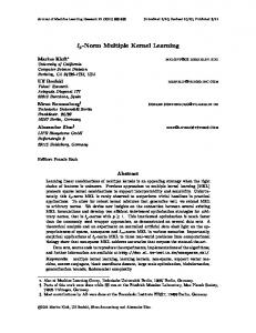
Varma & Babu, 2009; Vedaldi et al., 2009; Levinboim & Sha, 2012; Hwang et al., 2012). They have been demonstrated to be superior to a number of linear and non-linear filter and wrapper methods (Varma & Babu, 2009). MKL feature selection techniques were also used to reduce prediction time in the joint winning entry of the competitive PASCAL VOC 2009 object detection in images challenge (Vedaldi et al., 2009). However, even though many specialized MKL optimization techniques have been developed (Kloft et al., 2011; Vishwanathan et al., 2010; Orabona & Jie, 2011; Orabona et al., 2012; Jain et al., 2012), training them thousands of times with different parameter settings is often infeasible. Our objective, in this paper, is to develop MKL formulations and algorithms for efficiently determining the nonlinear feature selection path. Our starting point is a novel conjecture that, for certain MKL formulations subject to lp≥1 regularization, the number of features (kernels) selected in the optimal solution monotonically decreases as p is decreased from an initial value to unity. We first prove that the conjecture is true for a generic family of Kernel Target Alignment (KTA) based lp -MKL formulations. This implies that regulating p, in the formulations of this family, provides a principled way of generating the feature selection path (see Fig 1(a), 1(b)). In fact, for this family, we further strengthen the conjecture and prove that the feature weights themselves decay (grow) monotonically once they are below (above) a certain threshold at optimality (see Fig 1(c)-1(e)). This implies that there exist juncture points along the path and an algorithm can exploit these by eliminating certain features from the optimization for potentially large intervals of p. It should be noted that these conjectures are non-trivial and we show that they do not hold for the popular square loss based lp -MKL formulation. Based on these results, we propose a Generalized lp -KTA formulation which extends the KTA formulations of (Cristianini et al., 2001; Lanckriet et al., 2004; Cortes et al., 2012). The proposed formulation is strongly convex and leads to robust feature selection (Bousquet & Elisseeff, 2002; Zou & Hastie, 2005; Kivinen et al., 2006). Furthermore, the feature monotonicity results allow us to develop a predictor-corrector based path following algorithm for Generalized lp -KTA that exploits the presence of juncture points for increased efficiency. We perform extensive experiments to demonstrate that the proposed Generalized lp -KTA formulation can lead to classification accuracies which are as much as 10% higher on benchmark data sets not only as compared to other lp -MKL formulations and uniform kernel baselines but also leading feature selection methods. We further demonstrate that our algorithm reduces training time significantly over other path following algorithms and state-of-the-art lp -MKL op-
timizers such as SMO-MKL. In particular, we generate the entire feature selection path for data sets with a hundred thousand features in approximately half an hour on standard hardware. Entire path generation for such data set is well beyond the scaling capabilities of other methods. Our contributions are as follows: (a) we propose, and prove, a novel conjecture regarding the monotonicity of selected features, and feature weights themselves, for certain lp regularized MKL formulations; (b) we propose a Generalized lp -KTA formulation for robust non-linear feature selection that is capable of achieving significantly higher classification accuracies as compared to state-of-the-art; and (c) our algorithm is many times faster than other leading techniques.
2. Related Work Considerable progress has been made in the area of nonlinear feature selection. A popular approach is to map the input features to a kernel-induced feature space while simultaneously performing feature selection in the original input space. For example, (Li et al., 2006) propose to perform LASSO regression in the induced space and thereby perform non-linear feature selection while (Weston et al., 2000; Grandvalet & Canu, 2002) pose this problem as that of tuning the hyper-parameters of the kernel. Another promising direction is to find un-correlated or independent features in the kernel induced feature space. While (Wu et al., 2005; Cao et al., 2007) aim at selecting orthogonal features in the feature space, (Chen et al., 2008; Song et al., 2012) employ Hilbert-Schmidt Independence Criterion based measures. Most of these approaches are either computationally expensive or resort to approximately minimizing their non-convex objectives. Multiple Kernel Learning based techniques for nonlinear feature selection have been explored in settings such as multi-label classification (Ji et al., 2008), bioinformatics (Chen et al., 2008; Levinboim & Sha, 2012) and object categorization (Vedaldi et al., 2009; Hwang et al., 2012). In (Varma & Babu, 2009), MKL techniques for non-linear feature selection were shown to be better than boosting (Baluja & Rowley, 2007), lasso (Andrew & Gao, 2007), sparse SVM (Chan et al., 2007), LPSVM (Fung & Mangasarian, 2002) and BAHSIC (Song et al., 2012). Various MKL formulations have been developed including lp≥1 -norm regularization over the kernel weights (Lanckriet et al., 2004; Rakotomamonjy et al., 2008; Cortes et al., 2009a; Kloft et al., 2011; Orabona & Jie, 2011; Orabona et al., 2012), mixed-norm regularizers (Aflalo et al., 2011), non-linear combinations of base kernels (Cortes et al., 2009b; Varma & Babu, 2009), Bregman divergence based regularizers (Vishwanathan et al., 2010) and for regularized kernel discriminant analysis (Ye
Arcene Madelon Relathe Pcmac Basehock Dorothea
70 60 50 0
0.5 1 Fraction of Selected Features
0.8
4 0.6 Arcene Madelon Relathe Pcmac Basehock Dorothea
0.4 0.2 0 1
(a)
1.5 p
η < e−1 0.37
Feature 1 Feature 2 Feature 3 Feature 4
0.3
3
e−1 ≤ η < 1 0.65
Feature 5 Feature 6 Feature 7 Feature 8
Feature 9 Feature 10 Feature 11 Feature 12
0.6 0.55
0.2
η
80
5
η
Accuracy (%)
90
η≥1
1
η
100
Fraction of Selected Features
On p-norm Path Following in Multiple Kernel Learning for Non-linear Feature Selection
0.5 0.1
2
2
1 1
1.2
(b)
1.4
1.6
1.8
2
p
(c)
0 1
0.45 1.5 p
2
0.4 1
(d)
1.5 p
2
(e)
Figure 1: (a) The feature selection path for the proposed Generalized lp -KTA formulation. Note that generating the entire path for the largest data set (Dorothea) is well beyond the scaling capabilities of all existing algorithms while our proposed algorithm generated the path in only half an hour on standard hardware; (b) plot validating our weak Generalized lp -KTA monotonicity conjecture that the number of selected features decreases monotonically with p; (c) & (d) plots validating our strong Generalized lp -KTA monotonicity conjecture that feature (kernel) weights themselves vary monotonically beyond juncture points but vary non-monotonically in between (e). Figure best viewed in color under magnification. et al., 2008). State-of-the-art lp≥1 -MKL optimization techniques such as SMO-MKL (Vishwanathan et al., 2010) and SPG-GMKL (Jain et al., 2012) have been shown to scale to a million kernels. Nevertheless, these techniques take more than a day to train on a standard desktop and so computing them thousands of times for determining the entire feature selection path is infeasible. Path following over the regularization parameter has been studied in the context of both non-sparse regularization (Hastie et al., 2004) as well as sparse linear classifiers (Zhu et al., 2003). Some of the other settings where path following has been studied are: l1 -MKL (Bach et al., 2004), general non-linear regularization paths (Rosset, 2004), boosting (Zhao & Yu, 2007) and l1 regularized feature selection (Li & Sminchisescu, 2010). Tracing the solution path for other hyper-parameters has also been explored. While (Gunter & Zhu, 2005; Wang et al., 2006) perform path following over the tube width parameter in support vector regression, (Wang et al., 2007) follow the path for the kernel hyper-parameter in SVMs.
ing centered gram matrices obtained from the training data so that the features induced in the RKHS have zero mean (Cortes et al., 2012). Let y denote the vector with entries as the labels of the training data. We are interested in learning a kernel, k, thatP is a conic combination of the r given base kernels, i.e. k = i=1 ηi ki , ηi ≥ 0 ∀ i. We focus on the following family of Bregman divergence based lp -KTA formulations for learning the kernel weights η. Let F be a strictly convex and differentiable function and let ∇F denote its gradient. Then, the Bregman divergence generated by the function F is given by BF (x) = F (x) − F (x0 ) − (x − x0 )> ∇F (x0 ), where x0 is some fixed and given point in the domain of F . As an example, F (x) = hx, xi leads to BF (x) = kx − x0 k2 , the squared Euclidean distance. The proposed Generalized lp -KTA formulations have the following form: ¯F (η) + λ2 min λ1 B η≥0
r X i=1
ηip −
r X
ηi y> Ki y,
(1)
i=1
To the best of our knowledge, p-norm path following has not been studied in the literature so far. The closest competing technique to ours is the path following l1 -MKL approach of (Bach et al., 2004) and we present comparative results in Section 6.
where the first term representing the Bregman diver¯F (η) = gence based regularizer is decomposable as B P i BF (ηi ), the second term is the sparsity inducing lp regularizer and the third term captures the alignment of the learnt kernel to the ideal kernel yy> . Note that p ≥ 1, λ1 ≥ 0 and λ2 ≥ 0 are regularization parameters.
3. Generalized lp -KTA
A large number of popular Bregman divergences such as the squared Euclidean distance, generalized KL-divergence etc. are decomposable (Banerjee et al., 2005) and hence admissible under the Generalized lp -KTA formulation. Such Bregman divergences are known to promote robust feature and kernel selection (Bousquet & Elisseeff, 2002; Zou & Hastie, 2005; Kivinen et al., 2006) while the lp -norm regularizer achieves variable sparsity (Kloft et al., 2011). Note that the classical KTA formulations studied in (Lanckriet et al., 2004; Cristianini et al., 2001) can be obtained as special cases of our formulation by taking F to be the squared
To perform non-linear feature selection, we associate a non-linear base kernel with each individual feature, such as RBF kernels defined per feature, and then learn a sparse combination of base kernels. We introduce our Generalized lp -KTA formulation for sparse kernel learning using the following notation. Let k1 , . . . , kr denote the given base kernel functions (one per feature) and let K1 , . . . , Kr denote the correspond-
On p-norm Path Following in Multiple Kernel Learning for Non-linear Feature Selection
Euclidean distance and having λ2 = 0. On the other hand, substituting λ1 = 0 results in the KTA formulation studied in Proposition (7) in (Cortes et al., 2012). The normalized KTA formulation in Proposition (9) in (Cortes et al., 2012) employs a non-decomposable Bregman divergence and hence is not a special case of (1). However we empirically demonstrate in Section 6 that the proposed Generalized lp -KTA formulation outperforms this normalized KTA formulation both in terms of generalization accuracy as well as computational cost. In particular, the normalized KTA formulation needs to operate on an r × r dense matrix which becomes infeasible for large r (r = 105 for the standard Dorothea feature selection data set).
the gradient of the function at optimality, g 0 (ηi∗ ), should lie in the normal cone of the feasibility set (Ben-Tal & Nemirovski, 2001). This results in the following inequality:
The final classification results are obtained by training an Pr SVM using the learnt kernel k = i=1 ηi ki . This corresponds to non-linear feature selection since features for which ηi is zero do not contribute to the kernel and can be dropped from the data set.
F 0 (0) − F 0 (ηi0 ) = 0 and y> Ki y = 0
We conclude this section with the following observation. Though (1) optimizes the kernel weights independently for a given λ1 and λ2 , the proposed algorithm employs crossvalidation for optimizing λ2 . Hence, the final optimal kernel weights need not be independent.
(3)
Since F is a convex function, we have F (ηi ) ≥ F (ηi0 ) + F 0 (ηi0 )(ηi − ηi0 ) as well as F (ηi0 ) ≥ F (ηi ) + F 0 (ηi )(ηi0 − ηi ). Summing these two inequalities, we get 0 ≥ (F 0 (ηi )− F 0 (ηi0 ))(ηi0 − ηi ). Now substituting ηi = 0, we get 0 ≥ ηi0 (F 0 (0) − F 0 (ηi0 )). Since ηi0 ≥ 0 (feasible set of ηi is ≥ 0), it follows 0 ≥ F 0 (0) − F 0 (ηi0 ). Hence, in the LHS of (3), (F 0 (0) − F 0 (ηi0 )) ≤ 0 and −y> Ki y ≤ 0. It follows that the optimality conditions for ηi∗ = 0 are (4)
Note that both the above equalities are independent of p. It follows that if ∃ p0 > 1 s.t. ηi∗ (p0 ) = 0 then ηi∗ (p) = 0 ∀ p > 1. Thus, the optimal solution path, ηi∗ (p), is smooth, in fact constant, when ∃ p0 > 1 s.t. ηi∗ (p0 ) = 0. Case 2: ηi∗ > 0 for a given p: In this case, the necessary and sufficient conditions of optimality (Ben-Tal & Nemirovski, 2001) simplifies to g 0 (ηi∗ ) = 0. Thus we get the following optimality condition Gi (ηi , p) ≡λ1 (F 0 (ηi ) − F 0 (ηi0 )) + λ2 pηip−1
4. Monotonic Feature & Kernel Selection Path Following
− y> Ki y = 0
In this section, we prove the monotonicity conjecture for the proposed Generalized lp -KTA formulation. Let ηi∗ (p0 ) denote the optimal weight of the kernel ki obtained with (1) at p = p0 and let K(p0 ) denote the set of kernels active at p = p0 . A kernel ki is said to be active at p = p0 , i.e. ki ∈ K(p0 ). if and only if ηi∗ (p0 ) > �, where � > 0 is a user-defined tolerance. The proposed conjecture can now be formally stated as kj ∈ / K(p0 ) ⇒ kj ∈ / K(p) ∀ 1 < p < p0
λ1 (F 0 (0) − F 0 (ηi0 )) − y> Ki y ≥ 0
(2)
We begin our analysis by noting the following theorem: Theorem 1. The path of the optimal solutions of (1) with respect to p, i.e. η ∗ (p), is unique, smooth (provided F is twice-differentiable) and, in general, non-linear. Proof The optimal solution path of (1), i.e. η ∗ (p), is unique since the objective of (1) is strictly convex. In order to prove the smoothness of the optimal solution path, we begin by deriving the necessary and sufficient conditions of optimality for (1). To this end, we first define ¯F (ηi ) + λ2 η p − ηi y> Ki y g(ηi ) = λ1 B i Next, we consider two cases: Case 1: ηi∗ = 0 for a given p: The necessary and sufficient conditions of optimality for a convex function is that
(5)
In the following, we prove that the path of the optimal solution, ηi∗ (p), of (5) is smooth for the non trivial case: ηi∗ (p) > 0 ∀ p > 1. Since the pair (ηi∗ (p), p) always satisfy the in P equality ∂Gi (5), we must have that dGi (ηi∗ (p), p) ≡ j ∂ηj dηj + ∂Gi ∂p dp
= 0 ∀ p > 1. This leads to
−λ2 ηi∗ (p)p−1 (1 + p ln ηi∗ (p)) dηi∗ (p) = dp λ1 F 00 (ηi∗ (p)) + λ2 p(p − 1)ηi∗ (p)p−2
(6)
The terms ln ηi∗ (p) and ηi∗ (p)p−2 are always finite as ηi∗ (p) > 0 and the denominator of (6) is always nonzero, in fact positive, because for any convex, twicedifferentiable F we have: F 00 (ηi∗ (p)) ≥ 0. Hence, the derivative along the optimal solution path (6) is well defined and itself a continuous function; proving that the optimal solution path is smooth (but generally non-linear) in this case too. � The next theorem states the key result that proves the monotonicity conjecture for the proposed Generalized lp KTA formulation. Theorem 2. Given ηi∗ (p0 ), the following holds as p decreases from p0 to unity: (1) ηi∗ (p) decreases monotonically whenever ηi∗ (p0 ) < e−1 ; (2) ηi∗ (p) increases monotonically −1 whenever ηi∗ (p0 ) > e p0
On p-norm Path Following in Multiple Kernel Learning for Non-linear Feature Selection
Proof. The monotonic behavior of ηi∗ (p) follows from ob1 serving the sign of (6) and from the fact that e− p is a monotonically increasing function of p. Note that the denominator of (6) is positive. � Theorem 2 implies that the monotonicity conjecture for the Generalized lp -KTA formulation in (1) holds whenever the user defined tolerance parameter � (above which a kernel is said to be active) is set to be less than e−1 . Points wherever an optimal kernel weight becomes less than the threshold are referred to as juncture points. Note that Theorems 1,2 and the monotonicity conjecture are non-trivial as they do not hold for all loss functions. In particular, we analyze lp -MKL formulations with the popular square loss in Appendix A, and present settings where the conjecture does not hold. This implies that path following algorithms for such formulations can not be speeded up by eliminating features whose weights touch zero from the optimization since they can increase to become non-zero at a later stage (see Fig 2).
5. Efficient Path Following Algorithm In this section, we present an efficient path following algorithm which closely approximates the true feature selection path. The algorithm exploits the presence of juncture points to improve upon the standard Predictor-Corrector (PC) technique and scales effortlessly to optimization problems involving a hundred thousand features. Finally, we give a bound on the deviation from the optimal objective function value caused due to the approximation. Theorem 1 states that the solution path of (1) is smooth but non-linear in general. Path following is typically implemented using the standard Predictor-Corrector algorithm (Allgower & Georg, 1993) in such cases (Bach et al., 2004; Rosset, 2004). The PC algorithm is initialized with the optimal solution at p = p0 . At every iteration, the current value of p is decreased by a small step size, ∆p and the following key iterative steps are performed: Predictor: The predictor is a close approximation of ηi∗ (p − ∆p) given ηi∗ (p). This can either be the warm start approximation, i.e. ηi∗ (p − ∆p) = ηi∗ (p), the first order apdηi∗ (p) or the second proximation, ηi∗ (p−∆p) = ηi∗ (p)−∆p dp order approximation ηi∗ (p − ∆p) = ηi∗ (p) − ∆p 1 2
dηi∗ (p) dp
+
2 d2 η ∗ (p)
(∆p) dpi 2 (the derivative expressions for our case are provided in the supplementary material). Corrector: The Newton method is used to correct the approximations of the predictor step leading to a quadratic convergence rate (Allgower & Georg, 1993). We modify the standard PC algorithm so as to closely approximate the solution path at a lower computational cost. The key idea is to exploit the monotonicity in the active
Algorithm 1 Generic Algorithm for Computing Solution Path of the Kernel Weights Input: y> K1 y, . . . , y> Kr y, step size ∆p(> 0), tolerance �(> 0), start and end p values: p0 and pe respectively with p0 > p e . Output: η ∗ (p) for all p at ∆ intervals between [pe , p0 ] Initialization: p = p0 , Index set of active kernels K = {1, . . . , r} Solve (1) at p = p0 to obtain the optimal solution η ∗ (p0 ) if (ηi∗ (p0 )) < � for any i ∈ K then Set ηi∗ (p0 ) = 0 Update K = K \ {i} end if repeat Update p = p − ∆p Set ηi∗ (p) = 0 for all i ∈ /K for i ∈ K do Predictor: Initialize ηi∗ (p) using warm start or first or second order approximation Corrector: Run Newton’s method to obtain ηi∗ (p) end for if (ηi∗ (p)) < � for any i ∈ K then Set ηi∗ (p) = 0 Update K = K \ {i} end if until p ≤ pe
set size and directly set certain kernel weights to zero for all the subsequent p values. Algorithm 1 summarizes the proposed algorithm. The algorithm maintains an active-set that is initialized to those kernels whose optimal weight at p0 is above �. At every iteration, the first order PC step is used to determine the kernel weights for the next p value. Kernels whose weight falls below � are eliminated from the active set for the remainder of the optimization due to the monotonicity property. The error incurred by the proposed method can be bounded in terms of �. The following Lemma holds when the squared Euclidean distance is used as the Bregman divergence: Lemma 1. For any p, the deviation in the objective value of (1) obtained using the approximate path following algorithm from the true optimal objective is upper bounded by r(λ1 �2 + λ2 (p − 1)�p ). This result follows from the optimality conditions (5) and Theorem 2. We also state an analogous lemma for the generalized KL-divergence in the supplementary material.
Table 1: Data set statistics Data set Arcene Relathe Basehock
Num 100 1427 1993
Dim 10000 4322 4862
Data set Madelon Pcmac Dorothea
Num 2000 1943 800
Dim 500 3289 100000
On p-norm Path Following in Multiple Kernel Learning for Non-linear Feature Selection
Table 2: The maximum classification accuracy achieved (with the corresponding number of selected features) along the feature selection path. Generalized lp -KTA achieves significantly higher accuracies as compared to state-of-the-art KTA and lp≥1 -MKL formulations as well as leading feature selection techniques such as BAHSIC. The table reports mean results averaged over 5-fold cross validation (see the supplementary material for standard deviations). ‘-’ denote results where the data set was too large for the feature selection algorithm to generate results. Gen lp -KTA Centered-KTA SMO-MKL BAHSIC PF-l1 -MKL PF-l1 -SVM Uniform
Arcene 92.00 (3788) 75.00 (134) 82.00 (9999) 69.00 (100) 81.00 (87) 77.00 (273) 81.00 (10000)
Madelon 65.70 (12) 62.45 (290) 62.05 (1) 53.90 (50) 62.76 (89) 61.25 (7) 59.85 (500)
Relathe 92.57 (3644) 90.40 (542) 85.07 (500) 85.67 (287) 89.00 (510) 90.96 (4322)
Pcmac 93.62 (2947) 93.05 (498) 89.55 (500) 90.68 (190) 92.49 (3289)
Basehock 98.59 (4262) 97.29 (584) 93.58 (500) 97.24 (264) 97.99 (4862)
Dorothea 94.75 (20220) 90.63 (500) 93.88 (499) 91.38 (100000)
Table 3: The maximum classification accuracy achieved (with the corresponding number of selected features) along the feature selection path. In keeping with the ASU experimental protocol, all algorithms are restricted to selecting at most 200 features and are allowed to train on only half the data. Generalized lp -KTA (RBF) outperforms all the linear techniques and this demonstrates the advantages of non-linear feature selection. Amongst the linear methods, our proposed method with linear features is the best in general. Gen lp -KTA (RBF) Gen lp -KTA (Linear) Inf. Gain Chi-Square Fisher Score mRMR ReliefF Spectrum Gini Index K.-Wallis
Arcene 76.80 (124) 73.40 (16) 72.00 (110) 71.20 (120) 66.20 (65) 68.20 (60) 68.40 (170) 64.00 (195) 64.60 (185) 60.20 (95)
Madelon 64.50 (14) 62.04 (12) 61.63 (5) 61.69 (10) 61.47 (10) 61.87 (5) 62.06 (15) 60.19 (25) 59.43 (25) 55.04 (65)
Relathe 89.40 (183) 88.39 (190) 84.39 (190) 83.48 (180) 83.35 (180) 75.01 (60) 77.08 (200) 69.99 (175) 69.50 (180) 70.97 (200)
6. Experiments We carry out experiments to determine both the classification accuracy as well as the training time of the proposed Generalized lp -KTA over the feature selection path. Data sets & kernels: We present results on a variety of feature selection data sets taken from the NIPS 2003 Feature Selection Challenge (Guyon et al., 2006) and the ASU Feature Selection Repository (Zhao et al., 2010). Table 2 lists the number of instances and features in each data set. Unless otherwise stated, results are averaged via 5-fold crossvalidation (standard deviations are reported in the supplementary material for lack of space). We define an RBF kernel per feature as our base kernels and center and trace normalize them as recommended in (Cortes et al., 2012). Baseline techniques: We compare the proposed approach to a number of baseline techniques including state-of-theart Centered KTA formulation (Cortes et al., 2012), highly optimized lp -MKL techniques such as SMO-MKL (Vishwanathan et al., 2010), leading feature selection methods such as BAHSIC (Song et al., 2012) as well as path following approaches for l1 -MKL (PF-l1 -MKL) (Bach et al., 2004). While evaluating classification accuracy we also
Pcmac 89.76 (196) 88.88 (180) 88.99 (135) 88.24 (155) 88.02 (100) 83.34 (145) 80.76 (200) 66.74 (185) 66.60 (185) 65.20 (200)
Basehock 95.46 (184) 94.76 (189) 95.26 (200) 95.28 (160) 94.61 (200) 88.88 (70) 86.05 (200) 69.79 (200) 69.49 (200) 70.37 (200)
Dorothea 93.75 (17) 93.60 (12) 93.33 (35) 93.33 (20) 93.30 (20) 93.18 (155) 93.33 (105) 90.28 (140) 90.28 (140) 90.08 (65)
compare to the uniform kernel combination baseline (ηi = 1/r ∀ i) referred to as Uniform as well as path following linear feature selection approaches (PF-l1 -SVM) (Zhu et al., 2003). We also compare our classification accuracy to eight other state-of-the-art feature selection techniques whose details are given in Zhao et al. (2010). The final classification results for all the feature selection algorithms are obtained using an SVM with the kernel computed as Pr k = i=1 ηi ki , where (ηi )i=1,...,r are the feature weights provided by the algorithm. While evaluating computational cost, we also compare the cost of our proposed approximate first order predictor-corrector algorithm to the exact path following algorithm. Parameter settings: For the Generalized lp -KTA formulation we set λ1 , λ2 and the SVM misclassification penalty C by 5-fold cross-validation while varying p from 2 to 1 in decrements of 0.01. We use the squared Euclidean distance as the Bregman divergence with x0 = 0. BAHSIC, PFl1 -MKL and PF-l1 -SVM are parameter free when computing the feature selection path. The parameters of the other techniques were also set via extensive cross-validation except for the computationally intensive SMO-MKL where this was feasible only for the smaller data sets. On the
On p-norm Path Following in Multiple Kernel Learning for Non-linear Feature Selection
Table 4: Average training time (in seconds) required to compute a point along the feature selection path. Note that each algorithm generates a different number of points along the path. Therefore, for a fair comparison, we report the total time taken to compute the path for each algorithm divided by the number of points generated by the algorithm. Generalized lp KTA formulation is orders of magnitude faster than competing techniques and is the only algorithm which can generate the entire path for the Dorothea data set. ‘-’ denote results where the data set was too large for the feature selection algorithm to generate results. Gen lp -KTA Centered-KTA SMO-MKL BAHSIC PF-l1 -MKL
Arcene 0.3 10.9 5.7 116.2 29.5
Madelon 2.4 2405.5 168.4 2265.8 83.1
larger data sets, we follow the SMO-MKL’s authors’ experimental protocol and fix λ = 1 and validate over C with p ∈ {1.01, 1.33, 1.66, 2}. As in the case of previous lp MKL algorithms (Vishwanathan et al., 2010; Orabona & Jie, 2011; Orabona et al., 2012; Jain et al., 2012), we employ the common strategy of thresholding to obtain sparse solutions for the proposed Generalized lp -KTA. Results: Table 2 lists the maximum classification accuracy achieved along the entire feature selection path and the corresponding number of selected features (i.e. corresponding to the best oracle results on the test set). Our proposed Generalized lp -KTA formulation gets significantly higher classification accuracies than all competing methods. For instance, on Arcene data set, Generalized lp -KTA achieves a classification accuracy which is 10% higher than the closest competing method. Table 3 presents results obtained following the ASU experimental protocol where only 50% of the data is used for training and the number of selected features is restricted to be less than 200. This tests the capabilities of feature selection algorithms under the demanding conditions of both limited training data and limited prediction budget. As can be seen, Gen lp -KTA (RBF) clearly outperforms all the linear methods thereby demonstrating the power of non-linear feature selection which is the focus of our paper. Amongst all the linear feature selection methods, our proposed Gen lp -KTA (Linear) is the best in general. It is the best method on 3 data sets – on Relathe it is better than the second best method by 4%, on Arcene by 1.4% and on Dorothea by 0.27%. On 2 data sets it is the second best method – lagging behind the best method on Madelon by 0.02% and on Pcmac by 0.11%. These results demonstrate that the Generalized lp -KTA formulation can lead to better results not only as compared to other KTA and lp -MKL formulations but also as compared to leading feature selection techniques. Table 4 assesses the cost of computing the feature selection path. Note that algorithms such as BAHSIC compute the path a feature at a time while other algorithms, such PF-l1 -MKL, have a much sparser sampling of the path (in
Relathe 2.4 2093.8 3764.2 240.0
Pcmac 3.7 1099.6 5906 -
Basehock 4.8 3302.6 7847.1 -
Dorothea 12.5 10976.3 -
the limit Centered KTA produces only a single point on the path). Therefore, for a fair comparison, we report the total time taken by each algorithm divided by the number of points generated by it along the path. This measures the average time taken by each algorithm to generate a point along the path. Table 4 shows that the proposed approximate first order predictor-corrector algorithm can be 16 to 878 times faster than competing techniques. Furthermore, on the largest data set, Dorothea with 105 features, Centered-KTA, SMO-MKL and PF-l1 -MKL were not able to generate even a single point on the path whereas our algorithm was able to generate the entire path in 21 minutes using pre-computed kernels and 36 minutes using kernels computed on the fly. BAHSIC generates the path by adding a single feature at each iteration and was able to generate the initial path segment up to 500 features but at a high computational cost of more than 3 hours. All experiments were carried out on a standard 2.40 GHz Intel Xeon desktop with 32 GB of RAM. Finally, we note that our approximate path following algorithm was also found to be faster than the exact path following algorithm implemented with first order predictor or with warm restarts without exploiting juncture points and eliminating features from the optimization. The speedups against both the baselines varied with more than 3 times on Madelon and almost 4 times on Dorothea while the maximum relative deviation from the exact path was only 7.3×10⁻⁶ and 3.6×10⁻⁴ respectively. Figure 1(a) shows the feature selection path as computed by our approximate algorithm on all the data sets.
7. Conclusions We developed an efficient p-norm path following algorithm for non-linear feature selection in this paper. Our starting point was a novel conjecture that the number of selected features, and the feature weights themselves, vary monotonically with p in lp -MKL formulations. We proposed a Generalized lp -KTA formulation and proved that the conjecture holds for this formulation but not for other popular formulations such as the square loss based lp -MKL. The
On p-norm Path Following in Multiple Kernel Learning for Non-linear Feature Selection
monotonicity property of the Generalized lp -KTA formulation allows us to eliminate features whose weight goes below a certain threshold from the optimization for large intervals of p leading to efficient path following. It was theoretically and empirically demonstrated that this resulted in only a minor deviation from the exact path. Experiments also revealed that our proposed formulation could yield significantly higher classification accuracies as compared to state-of-the-art MKL and feature selection methods (by as much as 10% in some cases) and be many times faster than them. All in all, we were able to effortlessly compute the entire path for problems involving a hundred thousand features which are well beyond the scaling capabilities of existing path following techniques.
Acknowledgments
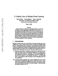
The proof involves deriving and analyzing the necessary conditions for the optimal value of a kernel weight in (7) to be zero and is detailed in the supplementary material. The above theorem shows a case in which the kernel weight, after attaining the lowest feasible value (zero), at p = p0 , grows as p further decreases from p0 . Figure 2 shows an instance from a real world data set (Parkinson disease data set from the UCI Repository) where the optimal kernel weight in (7) grows after attaining zero. We can observe that at around p = 1.5, the optimal kernel weight corresponding to Feature 1 is zero, and it again starts growing as p is further decreased. This observation shows that the conjecture is not universally true for low values of �. However, in the same setting as in Theorem 4, the conjecture may be true for some other � > 0. The proposed algorithm is usable whenever such an � is small1 .
We thank the anonymous reviewers for the valuable comments.
0.5 0.4
Feature 1 Feature 2
η
0.3
A. Analysis of lp -MKL with Square Loss
0.2
In this section, we analyze the proposed conjecture in the context of the lp -MKL formulation for the ridge regression (Cortes et al., 2009a): r X
1 ηip min maxm y> α − α> Qη α + λ2 η≥0 α∈R 2 i=1
(7)
P where Qη = i ηi Ki + 2λI 1 , I is the m×m identity matrix and λ1 , λ2 > 0 are the regularization parameters. Firstly, we consider a setting employed in (Lanckriet et al., 2004; Cristianini et al., 2001; 2000), which leads to the selection of a low-dimensional subspace: unit rank base kernels Ki = ui u> i s.t. trace(Ki ) = 1 and hKi , Kj i = 0 ∀ i 6= j. The following theorem holds in this setting: ηi∗ (p)
Theorem 3. Let denote the optimal weight corresponding to the i-th kernel in (7) at p. Given ηi∗ (p0 ), the following holds as p decreases from p0 to unity: (1) ηi∗ (p) decreases monotonically whenever ηi∗ (p0 ) < e−1 ; (2) ηi∗ (p) −1 increases monotonically whenever ηi∗ (p0 ) > e p0 The proof involves deriving and analyzing the dη ∗ (p)/dp term and is provided in the supplementary material. Needless to say, the above theorem implies that the conjecture is true for the case mentioned above. We now present an interesting example where the conjecture does not hold with � = 0: Theorem 4. Consider the regression formulation in (7) with two given base kernels of unit rank and unit trace: k1 and k2 . Additionally, let y> K2 K1 y > y> K1 y > 0. Then for some λ1 , λ2 , ∃ p0 > 1 such that η1 = 0 if and only if p = p0 .
0.1 0
1.2
1.4
1.6 p
1.8
2
Figure 2: η1∗ decrease as p is decreased from 2, attains zero at around p = 1.5 and again grows as p decreases further. This example proves that the monotonicity conjecture does not universally hold for (7) when � = 0.
In summary, the proposed conjecture is itself non-trivial and requires careful analysis for different lp -MKL formulations. Interestingly, in case of the proposed Generalized lp -KTA, it holds for small enough tolerance, � < e−1 .
References Aflalo, J., Ben-Tal, A., Bhattacharyya, C., Nath, J. Saketha, and Raman, S. Variable sparsity kernel learning. JMLR, 12:565– 592, 2011. Allgower, E. L. and Georg, K. Continuation and path following. Acta Numerica, 2:1–64, 1993. Andrew, G. and Gao, J. Scalable training of L 1-regularized loglinear models. In ICML, pp. 33–40, 2007. Bach, F. R. Exploring large feature spaces with hierarchical multiple kernel learning. In NIPS, pp. 105–112, 2008. Bach, F. R., Thibaux, R., and Jordan, M. I. Computing regularization paths for learning multiple kernels. In NIPS, 2004. Baluja, S. and Rowley, H. Boosting sex identification performance. IJCV, 71(1):111–119, 2007. 1 Interestingly, in our initial simulations on benchmark data sets, we found that many existing lp -MKL formulations do satisfy the conjecture at a reasonably low � > 0. We postpone theoretical analysis of this interesting and open question to future.
On p-norm Path Following in Multiple Kernel Learning for Non-linear Feature Selection Banerjee, A., Merugu, S., Dhillon, I. S., and Ghosh, J. Clustering with bregman divergences. JMLR, 6:1705–1749, 2005.
Kloft, M., Brefeld, U., Sonnenburg, S., and Zien, A. lp -norm multiple kernel learning. JMLR, 12:953–997, 2011.
Ben-Tal, A. and Nemirovski, A. Lectures on Modern Convex Optimization: Analysis, Algorithms and Engineering Applications. MPS/ SIAM Series on Optimization, 1, 2001.
Lanckriet, G. R. G., Cristianini, N., Bartlett, P., El Ghaoui, L., and Jordan, M. I. Learning the kernel matrix with semidefinite programming. JMLR, 5:27–72, 2004.
Bousquet, O. and Elisseeff, A. JMLR, 2:499–526, 2002.
Stability and generalization.
Levinboim, T. and Sha, F. Learning the kernel matrix with lowrank multiplicative shaping. In AAAI, 2012.
Cao, B., Shen, D., Sun, J. T., Yang, Q., and Chen, Z. Feature selection in a kernel space. In ICML, 2007.
Li, F. and Sminchisescu, C. The feature selection path in kernel methods. In AISTATS, 2010.
Chan, A. B., Vasconcelos, N., and Lanckriet, G. Direct convex relaxations of sparse SVM. In ICML, pp. 145–153, 2007.
Li, F., Yang, Y., and Xing, E. From lasso regression to feature vector machine. In NIPS, 2006.
Chen, J., Ji, S., Ceran, B., Li, Q., Wu, M., and Ye, J. Learning subspace kernels for classification. In KDD, 2008.
Orabona, F. and Jie, L. Ultra-fast optimization algorithm for sparse multi kernel learning. In ICML, 2011.
Cortes, C., Mohri, M., and Rostamizadeh, A. L2 regularization for learning kernels. In UAI, 2009a.
Orabona, F., Luo, J., and Caputo, B. Multi kernel learning with online-batch optimization. JMLR, 13:227–253, 2012.
Cortes, C., Mohri, M., and Rostamizadeh, A. Learning non-linear combinations of kernels. In NIPS, 2009b.
Rakotomamonjy, A., Bach, F., Grandvalet, Y., and Canu, S. SimpleMKL. JMLR, 9:2491–2521, 2008.
Cortes, C., Mohri, M., and Rostamizadeh, A. Algorithms for learning kernels based on centered alignment. JMLR, 13:795– 828, 2012.
Rosset, S. Following curved regularized optimization solution paths. In NIPS, 2004.
Cristianini, N., Lodhi, H., and Shawe-taylor, J. Latent semantic kernels for feature selection. Technical Report NC-TR-00-080, 2000. Cristianini, N., Shawe-Taylor, J., Elisseeff, A., and Kandola, J. On kernel-target alignment. In NIPS, 2001. Fung, G. and Mangasarian, O. L. A feature selection newton method for support vector machine classification. Technical Report 02-03, Univ. of Wisconsin, 2002.
Song, L., Smola, A., Gretton, A., Bedo, J., and Borgwardt, K. Feature selection via dependence maximization. JMLR, 13: 1393–1434, 2012. Varma, M. and Babu, B. R. More generality in efficient multiple kernel learning. In ICML, 2009. Vedaldi, A., Gulshan, V., Varma, M., and Zisserman, A. Multiple kernels for object detection. In ICCV, 2009.
Grandvalet, Y. and Canu, S. Adaptive scaling for feature selection in svms. In NIPS, 2002.
Vishwanathan, S. V. N., Sun, Z., Theera-Ampornpunt, N., and Varma, M. Multiple kernel learning and the smo algorithm. In NIPS, 2010.
Gunter, L. and Zhu, J. Computing the solution path for the regularized support vector regression. In NIPS, 2005.
Wang, G., Yeung, D.-Y., and Lochovsky, F. H. Two-dimensional solution path for support vector regression. In ICML, 2006.
Guyon, I., Gunn, S., Nikravesh, M., and Zadeh, L. A. Feature Extraction: Foundations and Applications. Springer-Verlag New York, Inc., 2006.
Wang, G., Yeung, D.-Y., and Lochovsky, F. H. A kernel path algorithm for support vector machines. In ICML, 2007.
Hastie, T., Rosset, S., Tibshirani, R., and Zhu, J. The entire regularization path for the support vector machine. JMLR, 5:1391– 1415, 2004. Hwang, S. J., Sha, F., and Grauman, K. Sharing features between objects and their attributes. In CVPR, pp. 1761–1768, 2011.
Weston, J., Mukherjee, S., Chapelle, O., Pontil, M., Poggio, T., and Vapnik, V. Feature selection for svms. In NIPS, 2000. Wu, M., Scholkopf, B., and Bakir, G. Building sparse large margin classifier. In ICML, 2005. Ye, J., , Ji, S., and Chen, J. Multi-class discriminant kernel learning via convex programming. JMLR, 9:719–758, 2008.
Hwang, S. J., Grauman, K., and Sha, F. Semantic kernel forests from multiple taxonomies. In NIPS, 2012.
Zhao, P. and Yu, B. Stagewise lasso. JMLR, 8:2701–2726, 2007.
Jain, A., Vishwanathan, S. V. N., and Varma, M. Spg-gmkl: Generalized multiple kernel learning with a million kernels. In KDD, 2012.
Zhao, Z., Morstatter, F., Sharma, S., Alelyani, S., Anand, A., and Liu, H. Advancing feature selection research. Technical report, Arizona State University, 2010.
Ji, S., Sun, L., Jin, R., and Ye, J. Multi-label multiple kernel learning. In NIPS, 2008.
Zhu, J., Rosset, S., Hastie, T., and Tibshirani, R. 1-norm Support Vector Machines. In NIPS, 2003.
Kivinen, J., Warmuth, M. K., and Hassibi, B. The p-norm generaliziation of the LMS algorithm for adaptive filtering. IEEE Trans. Signal Processing, 54(5):1782–1793, 2006.
Zou, H. and Hastie, T. Regularization and variable seclection via the elastic net. Journal of the Royal Statistical Society B, 67 (2):301–320, 2005.