The control chart based on geometric distribution (geometric chart) has been ... estimating the control limits of a geometric chart so that certain average run ...
Appeared in: Journal of Quality Technology, 2002, 34, 448-458.
1
On the Performance of Geometric Charts with Estimated Control Limits Z. Yanga, M. Xiea, V. Kuralmania and K.L. Tsuib a
National University of Singapore, Singapore 117543
b
Georgia Institute of Technology, Atlanta, Georgia, USA
Abstract The control chart based on geometric distribution (geometric chart) has been shown to be competitive to p- or np- charts for monitoring proportion nonconforming, especially for applications in high quality manufacturing environment. However, implementing a geometric chart often assumes the process parameter to be known or accurately estimated. For a high quality process, an accurate parameter estimate may require a very large sample size that is seldom available. In this paper we investigate the sample size effect when the process parameter needs to be estimated. It is shown that the estimated control limits create dependence among the monitoring events. Analytical approximation is derived to compute shift detection probabilities and run length distributions. It is found that, when there is no shift in proportion nonconforming, the false alarm probability increases as the sample size decreases and the effect can be significant even with sample size as large as 10,000. However, the in-control average run length is only affected mildly. On the other hand, when there is a process shift, the out-of-control average run length can be significantly affected by the estimated control limits, even with very large sample sizes. In practice, the quantitative results of the paper can be used to determine the minimum number of items required for estimating the control limits of a geometric chart so that certain average run length requirements are met.
Keywords: Geometric chart, estimated control limits, false alarm probability, average run length, sample size determination, high-quality processes, cumulative count of conforming items
Appeared in: Journal of Quality Technology, 2002, 34, 448-458.
2
1. Introduction Statistical process control has been shown to be very effective in monitoring and improving manufacturing and service processes. In practice, implementing a control chart often assumes the process parameters to be known or accurately estimated so that the control limits can be computed. For high quality processes, an accurate parameter estimate may require a very large sample size that is seldom available. It is important to understand the impact of the estimated control limits when the process parameters have to be estimated so that the size of the inspected sample can be determined. For monitoring normal data, Hillier (1969) pioneered the research on the estimated control limits for the X and R charts. Quesenberry (1993) further studied the effects of the sample size on estimated limits for X and X charts. Other related studies can be found in Proschan and Savage (1960), Nelson (1984), Quesenberry (1991), Montgomery (1996), Chen (1997, 1998) and Braun (1999). This paper investigates the effect of estimating control limits on the geometric chart, a statistical control chart that is shown to be particularly useful for high quality processes (Kaminsky et al., 1992, Glushkovsky, 1994, Nelson, 1994, Woodall, 1997, Xie and Goh, 1992, 1997). By monitoring cumulative count of conforming items between two nonconforming ones, we could detect further process improvement (Goh and Xie, 1994), avoid the problem of fixing the rational sample size, and reduce the amount of plotting. However, it is especially important to study the effect of estimated control limit in this case as for high quality processes, nonconforming items are rare and a very large sample size is needed to obtain a reasonably accurate estimate of the parameters. The error in the estimated fraction nonconforming p could possibly lead the estimated control limits to be far from the true limits. Under such circumstances, the misleading results as indicated by the geometric chart may result in wrong management decisions. In fact, the study of estimated control limits is a general research issue of importance (Woodall and Montgomery, 1999). The paper is organized as follows. First the geometric chart with a known or estimated process parameter is described and the problem of estimation error is discussed. The effect of
Appeared in: Journal of Quality Technology, 2002, 34, 448-458.
3
estimating control limits is then investigated and compared with the case of known limits for geometric chart. Explicit equations for false alarm probability and run length distribution are derived. The minimum sample size that provides the geometric chart the protection against giving misleading results is then discussed.
2. The Geometric Charts with Known or Estimated Model Parameter Let Yi be the cumulative count of conforming items between the (i-1)th and ith nonconforming items, from a stable process running in an automated manufacturing environment with the probability of having a nonconforming item p0. As a stable process is just a sequence of independent Bernoulli trials with the same probability of success p0, Yi + 1 is distributed as geometric with parameter p0. Hence the probability mass function of Yi is
g ( yi ) = (1 − p0 ) yi p0 , yi = 0, 1, … , with P (Yi ≥ y i ) = (1 − p0 ) yi . Let LCL and UCL be, respectively, the lower and upper probability control limits for Yi. Then LCL and UCL must satisfy, LCL −1
∑ (1 − p0 ) yi p0 =
yi =0
α 2
∞
and
∑ (1 − p0 ) y
i
yi =UCL +1
p0 =
α 2
,
which are equivalent to 1 − (1 − p0 ) LCL =
α 2
and (1 − p0 )UCL+1 =
α 2
.
Thus, the control limits for the geometric chart have the form: LCL =
ln(1 − α 2) , and ln(1 − p0 )
(1)
UCL =
ln(α 2) − 1. ln(1 − p0 )
(2)
Appeared in: Journal of Quality Technology, 2002, 34, 448-458.
4
It should be noted that these limits produce roughly the desired α for sufficient small p0, but not exact due to the discrete nature of the geometric distribution. In this sense, α may be understood as the overall desired false alarm rate. The true false alarm rate may deviate a bit from it, but our calculations (Table 1) show that this deviation is negligible. These formulas assume that the fraction nonconforming p0 is known. If it is not known, a common practice is to inspect an initial number of nonconforming items and estimate the fraction nonconforming value. An accurate estimate requires a large sample size, and usually because of the estimation error due to small sample size, the estimated control limits could be far from the exact values. When p0 is unknown but an initial sample is taken, the traditional estimate is pˆ 0 =
N , m
where N is the number of nonconforming items among a total of m items sampled. Clearly, N ~ Binomial(m, p0 ). Using pˆ 0 as an estimate of p0 , we obtain estimated control limits for the geometric chart:
LCˆ L( N ) =
ln(1 − α 2) , and ln(1 − N / m)
(3)
UCˆ L( N ) =
ln(α 2) − 1. ln(1 − N / m)
(4)
The aim in this paper is to investigate the performance of (3) and (4).
3. The Alarm Rate When the Parameters are Estimated Let Yi be a future observation (number of conforming items between two adjacent nonconforming items) from a process (possibly shifted from p0 to p). Define the event, Bi = { Yi > UCˆ L( N ) or Yi < LCˆ L( N ) }.
Appeared in: Journal of Quality Technology, 2002, 34, 448-458.
5
Then, P( Bi ) is the actual alarm rate (AR), which becomes the actual false alarm rate (FAR) when p = p 0 . Following a conditional argument, we obtain m m ⎛m⎞ P ( Bi ) = ∑ P( Bi | N = n)P( N = n) = ∑ P( Bi | N = n)⎜ ⎟ p 0n (1 − p 0 ) m − n ⎝n⎠ n =0 n =0
(5)
where P ( Bi | N = n) = P{ Yi > UCˆ L( N ) | N = n} + P{Yi < LCˆ L( N ) | N = n} = (1 − p) ln(α 2 ) ln(1−n m ) − (1 − p ) ln(1−α
2) ln(1− n m )
+ 1.
(6)
Notice that the events Bi ’s are dependent of each other, as they all depend on the same estimated control limits. Lai et al. (1998) considered the effects of data correlation on the geometric chart procedure, but did not consider the effect of estimation. So, the actual AR or FAR can be calculated using (5). To simplify the computation, a truncation procedure is given in the Appendix and it has been shown to be accurate and efficient. Table1 provides FAR values for different combinations of p 0 and m, and Table 2 provides AR values when the process parameter is shifted from p 0 = 0.0005. It is apparent from Table 1 that the actual FAR can deviate a lot from its desired value of 0.0027 when the true process fraction nonconforming p 0 is estimated from m sampled items, especially when p 0 is very small. For a fixed p 0 value, increasing m will significantly reduce the amount of deviation. This is because the variability in the estimated p 0 gets smaller as m increases. When sample size m is large enough (a smaller p 0 requires a larger m), the FAR can be very close to 0.0027, and hence the estimation effects on the false alarm probability of the geometric chart can be neglected. For example, when p 0 = 0.0001 and m = 800,000, we have FAR = 0.00297 and when p 0 = 0.001 and m = 100,000, we have FAR = 0.00292. Thus, for a high quality manufacturing process, i.e., when it is known that p 0 is small, Table 1 may be used for deciding an appropriate sample size for implementing a Gchart. Finally, it should be pointed out that even if the true p 0 value is used in the control limits, the FAR is still not exactly 0.0027 as the distribution is discrete.
Appeared in: Journal of Quality Technology, 2002, 34, 448-458.
6
Table 1. Values of FAR for G-Chart with Estimated Control Limits, α = 0.0027. m \ p0 10000
0.0001 0.0002 0.0003 0.0004 0.0005 0.0006 0.0007 0.0008 0.0009 0.001 0.38651 0.14718 0.05911 0.02623 0.01371 0.00878 0.00671 0.00575 0.00524 0.00492
20000
0.14719 0.02623 0.00878 0.00575 0.00492 0.00452 0.00425 0.00406 0.00391 0.00379
50000
0.01372 0.00492 0.00415 0.00379 0.00357 0.00343 0.00332 0.00325 0.00319 0.00314
100000 0.00492 0.00379 0.00343 0.00325 0.00314 0.00306 0.00301 0.00297 0.00294 0.00292 200000 0.00378 0.00324 0.00306 0.00297 0.00291 0.00288 0.00286 0.00283 0.00282 0.00281 300000 0.00343 0.00306 0.00294 0.00288 0.00284 0.00282 0.00281 0.00279 0.00278 0.00277 400000 0.00324 0.00297 0.00288 0.00283 0.00281 0.00279 0.00278 0.00277 0.00276 0.00276 500000 0.00314 0.00292 0.00285 0.00281 0.00279 0.00277 0.00276 0.00276 0.00275 0.00275 600000 0.00306 0.00288 0.00282 0.00279 0.00279 0.00277 0.00276 0.00275 0.00274 0.00274 700000 0.00301 0.00286 0.0028 0.00278 0.00276 0.00275 0.00275 0.00274 0.00274 0.00273 800000 0.00297 0.00284 0.00279 0.00277 0.00276 0.00275 0.00274 0.00274 0.00273 0.00273 900000 0.00294 0.00282 0.00278 0.00276 0.00274 0.00274 0.00274 0.00273 0.00273 0.00273 1000000 0.00292 0.00281 0.00277 0.00276 0.00274 0.00273 0.00273 0.00273 0.00273 0.00272 2000000 0.00281 0.00276 0.00274 0.00273 0.00272 0.00272 0.00272 0.00272 0.00271 0.00271 ∞
0.00270 0.00270 0.00270 0.00270 0.00270 0.00270 0.00270 0.00270 0.00270 0.00270
From Table 2, we see that for a given p ≠ p 0 (i.e., a given shifted process), the AR behaves similarly to the FAR as m increases, i.e., converging to its known value. For a given m, the AR increases as p decreases, but as p increases it first decreases and then increases very slowly. This means that G-chart is able to detect a process improvement (p decreases), but is unable to detect a process deterioration unless the deterioration amount is large enough. This seems to be a common problem for a probability chart of a quantity having a skewed distribution (See Xie and Goh, 1997), irrespective whether the control limits are known or estimated. The explanation is simple for a G-chart of a high yield process. As p 0 is small, the LCL is usually very small (e.g., 2.7 for α = 0.0027 and p 0 = 0.0005). When p is decreased, the plotted quantity Y tends to be larger, hence more chance to exceed UCL, resulting in an increased AR. When p is increased, the plotted quantity tends to be smaller, hence less chance to exceed UCL. At the same time, the chance for the plotted quantity to go below LCL would not increase much as LCL is already very small, unless p is increased by a big amount. This is why AR decreases first and slowly increases when p moves to right of p0. Other values of p0 were also examined and the general conclusions reached are consistent.
Appeared in: Journal of Quality Technology, 2002, 34, 448-458.
7
Table 2. Values of AR for G-Chart with Estimated Control Limits: a. α = 0.0027, p0=0.0005 m \p 10000
0.0001 0.0002 0.0003 0.0004 0.0005 0.0006 0.0007 0.0008 0.0009 0.001 0.25860 0.09028 0.03854 0.02047 0.01371 0.01114 0.01023 0.01000 0.01009 0.01031
20000
0.25751 0.07797 0.02648 0.01027 0.00492 0.00317 0.00270 0.00270 0.00288 0.00313
50000
0.26268 0.07421 0.02264 0.00786 0.00357 0.00241 0.00222 0.00234 0.00257 0.00283
100000 0.26479 0.07296 0.02126 0.00702 0.00314 0.00219 0.00209 0.00226 0.00250 0.00276 200000 0.26592 0.07234 0.02054 0.00658 0.00292 0.00208 0.00203 0.00222 0.00247 0.00273 300000 0.26631 0.07213 0.02029 0.00640 0.00285 0.00205 0.00202 0.00221 0.00246 0.00272 400000 0.26650 0.07203 0.02017 0.00637 0.00281 0.00203 0.00201 0.00220 0.00245 0.00271 500000 0.26662 0.07197 0.02010 0.00632 0.00278 0.00202 0.00200 0.00220 0.00245 0.00271 600000 0.26670 0.07190 0.02005 0.00629 0.00277 0.00201 0.00200 0.00220 0.00245 0.00271 700000 0.26676 0.07190 0.02001 0.00627 0.00276 0.00200 0.00200 0.00219 0.00244 0.00271 800000 0.26680 0.07188 0.01998 0.00626 0.00276 0.00200 0.00200 0.00219 0.00244 0.00271 900000 0.26683 0.07186 0.01996 0.00624 0.00274 0.00200 0.00200 0.00219 0.00244 0.00271 1000000 0.26686 0.07185 0.01995 0.00623 0.00274 0.00200 0.00200 0.00219 0.00244 0.00271 ∞
0.26707 0.07171 0.01979 0.00614 0.00270 0.00198 0.00199 0.00219 0.00244 0.00270
10000
0.17323 0.07859 0.05911 0.05439 0.05336 0.05339 0.05376 0.05424 0.05477 0.05531
20000
0.11968 0.02467 0.00878 0.00586 0.00559 0.00592 0.00641 0.00695 0.00750 0.00806
50000
0.11317 0.01713 0.00415 0.00244 0.00253 0.00293 0.00340 0.00388 0.00436 0.00484
b. α = 0.0027, p0=0.0003
100000 0.11197 0.01521 0.00342 0.00218 0.00238 0.00280 0.00326 0.00372 0.00419 0.00465 200000 0.11145 0.01419 0.00306 0.00206 0.00232 0.00275 0.00320 0.00366 0.00412 0.00457 300000 0.11129 0.01384 0.00294 0.00202 0.00230 0.00273 0.00318 0.00364 0.00409 0.00454 400000 0.11121 0.01366 0.00288 0.00200 0.00229 0.00272 0.00317 0.00363 0.00408 0.00453 500000 0.11117 0.01355 0.00285 0.00199 0.00229 0.00272 0.00317 0.00362 0.00407 0.00452 600000 0.11111 0.01347 0.00282 0.00198 0.00228 0.00271 0.00317 0.00362 0.00407 0.00452 700000 0.11111 0.01343 0.00280 0.00197 0.00228 0.00271 0.00316 0.00361 0.00407 0.00452 800000 0.11110 0.01339 0.00279 0.00196 0.00228 0.00271 0.00316 0.00361 0.00406 0.00451 900000 0.11109 0.01336 0.00278 0.00197 0.00227 0.00271 0.00316 0.00361 0.00406 0.00451 1000000 0.11108 0.01333 0.00277 0.00197 0.00228 0.00271 0.00316 0.00361 0.00406 0.00451 ∞
0.11100 0.01312 0.00270 0.00195 0.00227 0.00270 0.00315 0.00360 0.00405 0.00449
10000
0.36599 0.15356 0.06989 0.03408 0.01790 0.01033 0.00671 0.00499 0.00421 0.00390
20000
0.37621 0.15164 0.06444 0.02881 0.01369 0.00712 0.00425 0.00302 0.00255 0.00243
50000
0.38394 0.15156 0.06152 0.02585 0.01149 0.00566 0.00332 0.00244 0.00216 0.00216
c. α = 0.0027, p0=0.0007
100000 0.38664 0.15166 0.06051 0.02479 0.01070 0.00515 0.00301 0.00225 0.00205 0.00208 200000 0.38801 0.15175 0.06002 0.02425 0.01030 0.00489 0.00286 0.00216 0.00199 0.00204 300000 0.38847 0.15178 0.05984 0.02408 0.01016 0.00480 0.00280 0.00213 0.00197 0.00203 400000 0.38870 0.15179 0.05977 0.02398 0.01009 0.00476 0.00278 0.00211 0.00197 0.00202 500000 0.38884 0.15180 0.05972 0.02392 0.01005 0.00473 0.00276 0.00210 0.00196 0.00202 600000 0.38893 0.15181 0.05968 0.02389 0.01002 0.00472 0.00275 0.00210 0.00196 0.00202 700000 0.38900 0.15182 0.05966 0.02386 0.01000 0.00470 0.00274 0.00209 0.00195 0.00201 800000 0.38905 0.15182 0.05964 0.02384 0.00999 0.00469 0.00274 0.00209 0.00195 0.00201 900000 0.38908 0.15182 0.05963 0.02383 0.00998 0.00469 0.00274 0.00209 0.00195 0.00201 1000000 0.38912 0.15183 0.05962 0.02381 0.00997 0.00468 0.00273 0.00209 0.00195 0.00201 ∞
0.38939 0.15185 0.05952 0.02370 0.00989 0.00463 0.00270 0.00207 0.00194 0.00201
Appeared in: Journal of Quality Technology, 2002, 34, 448-458.
8
4. Run Length Distribution with Estimated Limits Let R be the number of points plotted on the chart until an out-of-control signal is given. The R is called the run length and the distribution of R is called the run length distribution. The study of run length distribution for a given control chart is of a great interest to quality professionals, especially when the events are correlated and/or the control limits are estimated. Denote P( Bi | N ) defined in (6) by α (N ) . It is easy to see that the conditional distribution of R given N is geometric with parameter α ( N ) . Hence, the unconditional distribution of R is: m
f R (r; p0 , p) =
∑ [1 − α (n)]r −1α (n)P( N = n)
n =0
⎛m⎞
m
=
∑ [1 − α (n)]r −1α (n)⎜⎝ n ⎟⎠ p0n (1 − p0 ) m−n
(7)
n =0
The run length distribution given in (7) can be easily evaluated and plotted, for any p0 and p, using Mathematica or some other statistical software. Figure 1 shows the run length distribution with p= p0 = 0.0005 and three different sample sizes. It is seen that the three run length distributions differ mainly in the left tail, a smaller m results in a taller curve in the left tail. This means that more short runs are to be expected.
0.008 m=10000
0.007
m=50000
0.006
m=100000
f(r)
0.005 0.004 0.003 0.002 0.001 0 0
100
200
300
400
500
600
700
800
900
1000
Run length(r)
Fig.1: Run length Distribution for three different sample sizes, p= p0 = 0.0005.
Appeared in: Journal of Quality Technology, 2002, 34, 448-458.
9
Following the similar conditional arguments, the average run length (ARL) and the standard deviation of the run length (SDRL) can be seen to have the forms:
ARL( p0 , p) = E N [1 α ( N )] , and
(8)
SDRL( p0 , p ) = VarN [1 α ( N )] + E N [(1 − α ( N )) α 2 ( N )] .
(9)
Thus, using the distribution of N, the quantities involved in (8) and (9) can be calculated as: 1 ⎛m⎞ n m−n , and ⎜ ⎟ p 0 (1 − p0 ) n = 0 α ( n) ⎝ n ⎠ m
E N [1 / α ( N )] = ∑
1 ⎛m⎞ n m−n . ⎜ ⎟ p 0 (1 − p 0 ) 2 ( n ) α n ⎝ ⎠ n =0 m
E N [1 / α 2 ( N )] = ∑
The corresponding ARL and SDRL with known control limits are of the forms ARL0 ( p0 , p) = 1 / P( Ai ) , and SDRL0 ( p0 , p ) = 1 − P( Ai ) / P( Ai ) =
(10) ARL( ARL − 1) ,
(11)
where the events Ai are defined similarly as Bi, but correspond to the known control limits. � � Thus, a reasonable way to decide when the sample size m is large enough for UCL and LCL to be essentially the same as UCL and LCL is to determine when the ARL and SDRL with estimated control limits are essentially the same as those given in (10) and (11). For instance, for α = 0.0027 and p = p0, one should have ARL ≅ SDRL ≅ 370. To study the effect of the sample size m on the mean and standard deviation (ARL and SDRL) of the run length distribution, values of ARL and SDRL are computed from Equations (8) and (9) for a range of values of m and p and for a fixed p0 = 0.0005 . For each value of p and m, the first value given is the ARL and the second is the SDRL. For comparison purpose, the exact values for the known p case are given in the last row ( m = ∞ ). Comparing the values in Table 3 with their nominal values, certain observations can be noted. First, estimating control limits can cause both ARL and SDRL larger or smaller than their
Appeared in: Journal of Quality Technology, 2002, 34, 448-458.
10
nominal levels, depending on whether p is smaller or larger than p0. This is due to the reduced or enlarged probabilities of events {Bi } and the dependence among them. Also, for large values of m, SDRL can exceed ARL, which is in contrast of the case of known control limits where SDRL =
ARL( ARL − 1) < ARL .
Considering the nature of the run length distribution, it can be seen that when SDRL exceeds ARL, a large number of short runs that are balanced by a few long runs would be expected, when compared with the standard geometric distribution.
This is because when two
probability distributions have the same mean, the one with larger standard deviation will have higher probability in its tails. Since the run length takes only the values that are positive integers, which cannot be less than 1, this means that the probability on the lower integers of the distribution with large standard deviation has to be increased and be balanced by an increase in the probability on large integers in the right tail of the distribution. The net effect of the dependence caused by using the estimated control limits UCˆ L and LCˆ L is that the run length distribution will, for a particular value of ARL, have an increased rate of very short runs between alarm signals. There will also be an increased number of long runs between alarm signals. However, the ratio of the number of short runs to the number of long ones also increases and is very large itself.
This is an undesirable phenomenon one should be
constantly aware of. Similar to the behavior of AR function with respect to a change in p, the ARL and SDRL both decrease as p decreases, but when p increases, ARL and SDRL both increase first and then decrease. The latter phenomenon is undesirable and can be explained in the same way as for AR function. By comparing Tables 2 and 3, it is interesting to note that the impact of estimated control limits are very different on the FAR and the in-control ARL (i.e., p0=0.0005). While the FAR in Table 2 significantly increases as the sample size decreases, the in-control ARL's are only affected mildly by the sample size. On the other hand, the out-of-control ARL's in Table 3 are very significantly affected as the sample size decreases, even with very large sample sizes.
Appeared in: Journal of Quality Technology, 2002, 34, 448-458.
11
Table 3. Values of ARL (upper entry) and SDRL (lower entry) for the G-Chart with Estimated Control Limits, p0 = 0.0005 M \ p 0.0001 0.0002 0.0003 10000 95.05 173.62 262.73 18.55 64.10 138.51 20000 29.42 108.72 221.54 6.56 37.08 114.24 50000 4.50 34.67 134.84 4.18 19.38 78.43 100000 3.61 19.18 87.26 3.93 16.02 63.25 200000 3.38 15.65 65.55 3.83 14.87 56.33 300000 3.32 14.81 59.63 3.80 14.54 54.26 400000 3.29 14.43 56.96 3.79 14.38 53.27 500000 3.27 14.22 55.45 3.78 14.29 52.70 600000 3.26 14.08 54.47 3.77 14.23 52.32 700000 3.25 13.98 53.79 3.77 14.19 52.05 800000 3.25 13.91 53.29 3.77 14.16 51.85 900000 3.24 13.86 52.91 3.76 14.13 51.70 1000000 3.24 13.81 52.61 3.76 14.11 51.58 2000000 3.75 14.03 51.04 3.22 13.62 51.28 3.74 13.95 50.52 ∞ 3.21 13.44 50.02
0.0005 0.0004 0.0006 0.0007 0.0008 0.0009 331.3 374.1 397.5 406.9 406.0 397.1 221.4 291.8 339.1 362.3 366.0 356.7 323.8 391.6 426.2 436.4 429.0 410.1 224.1 326.2 391.0 414.4 408.4 386.7 281.3 398.8 457.4 467.6 447.9 415.1 206.8 353.0 442.0 460.8 439.0 403.6 239.5 394.8 474.9 483.4 454.0 414.0 190.4 362.9 467.8 480.9 449.1 407.8 205.6 387.6 487.1 492.8 456.2 412.4 178.1 367.5 484.3 492.0 453.7 409.3 191.9 383.4 492.2 496.2 456.7 411.7 173.3 368.7 490.7 495.8 455.1 409.8 184.7 380.8 494.9 497.9 456.9 411.3 170.8 369.2 494.0 497.8 455.8 410.0 180.3 379.0 496.7 498.9 457.0 411.1 169.2 369.5 496.1 498.9 456.2 410.1 177.3 377.7 497.9 499.6 457.0 410.9 168.2 369.7 497.5 499.7 456.4 410.2 175.1 376.7 498.8 500.1 457.1 410.8 167.4 369.8 498.6 500.3 456.6 410.2 173.5 376.0 499.5 500.5 457.1 410.7 166.8 369.9 499.3 500.7 456.7 410.3 172.3 375.4 500.0 500.8 457.1 410.6 166.4 369.9 500.0 501.00 456.9 410.3 171.3 374.9 500.4 501.0 457.1 410.6 166.0 370.0 500.4 501.3 456.9 410.3 164.4 370.2 502.7 502.4 457.3 410.4 166.8 372.5 502.4 502.1 457.1 410.3 162.8 370.4 505.1 503.1 457.7 410.5 162.3 369.9 504.6 503.1 457.2 410.0
0.001 382.7 340.1 385.4 359.5 380.2 367.9 375.8 369.4 373.0 370.0 372.0 370.1 371.4 370.1 371.3 370.2 370.9 370.2 370.7 370.2 370.6 370.2 370.5 370.2 370.5 370.2 370.3 370.1 370.3 369.8
5. Alternative Measures of Run Length Tables 2 and 3 exhibit some undesirable behavior: the G-chart is unable to detect the process deterioration. It should be pointed out that this is not induced by estimating the control limits, but rather an artifact of the geometric chart. This point can clearly be seen by comparing the results in the last rows of Tables 2 and 3 with results in the other rows. The run length is defined as the number of plotted points until an out-of-control signal. In other words, it is the number of consecutive nonconforming items until an out-of-control signal. However, what really matters is the total number of checked items Rt until an out-ofcontrol signal. Using the earlier notation, the ith plotted point corresponds to Wi = Yi+1 checked items and Wi tends to be larger when p is smaller and smaller when p is larger. Clearly, R t = ∑ iR=1 W i and
Appeared in: Journal of Quality Technology, 2002, 34, 448-458.
12
E ( R t ) = E[ E ( R t N )] = E[ E (∑ iR=1 W i N )] = E[ E ( R N ) E (W i N )] . The last equation follows Wald’s Identity. As Wi is independent of N, we have ARLt = E ( R t ) = E[ E ( R N ) p] = ARL p . As Rt is defined in terms of number of inspected items, the ARLt is referred to as the average run length per item. Using above relation, one can easily convert the results in Table 3 into the values of ARLt. The converted results are given in Table 4. From the results in Table 4, we see that for smaller values of m (i.e., less than 100000) average run lengths per item ARLt decrease after the .0005 entry. For larger values of m, the ARLt begin to decrease after the .0006 entry.
This means that using ARLt one is able to
detect the process deterioration. On the other hand, the ARLt to the left of the .0005 entry increases when m =10000. This is clearly a consequence of estimation. For larger values of m, the ARLt to the left of the .0005 entry usually decrease, which is what one would expect. Similar results can be obtained for alarm rates per item. (Multiply the original alarm rates by p.) The SDRL can also be dealt with but the transformation is a bit more complicated. In summary, G-chart is able to detect both decrease and increase in fraction nonconforming if one uses the run length measures introduced above. Recently, Wu and Spedding (2001) introduced a synthetic control chart for detecting fraction nonconforming increase. Table 4. The Average Run Length Per Item M\ p
0.0001
0.0002
0.0003
0.0004
0.0005
0.0006
0.0007
0.0008
0.0009
0.001
10000
950520
868100
875780
828120
748170
662470
581346
507470
441244
382655
20000
294150
543580
738470
809412
783106
710407
623360
536193
455714
385411
50000
44960
173355
449473
703335
797504
762323
668023
559826
461208
380216
100000
36050
95880
290877
598635
789590
791467
690497
567451
460019
375816
200000
33820
78255
218497
513890
775134
811902
703981
570228
458262
372987
300000
33190
74055
198777
479703
766788
820272
708804
570849
457470
371956
400000
32890
72165
189867
461670
761558
824870
711263
571085
457033
371426
500000
32710
71090
184820
450622
757998
827787
712749
571201
456759
371103
600000
32600
70395
181573
443182
755422
829802
713741
571266
456571
370886
700000
32520
69905
179311
437840
753476
831280
714453
571308
456433
370730
800000
32460
69550
177645
433820
751954
832410
714986
571335
456330
370612
900000
32410
69275
176367
430690
750732
833302
715400
571354
456248
370521
1000000
32380
69055
175356
428180
749728
834025
715733
571369
456181
370447
2000000
37520
70130
170122
410958
740318
837847
717760
571623
456013
370253
37440
69725
168406
406983
740740
841835
719454
572076
456123
370279
∞
Appeared in: Journal of Quality Technology, 2002, 34, 448-458.
13
6. Conclusions Geometric control chart is useful in different context (Kaminsky et al., 1992, Nelson, 1994, Glushkovsky, 1994, Benneyan and Kaminsky, 1994, and Benneyan, 2001). However, it is particularly useful when the cumulative count of conforming items between two nonconforming ones is monitored for high quality process. This poses a great challenge, as the estimation error could be significant when the sample size is not large enough. In this paper we show that the estimated control limits create dependence among the monitoring events. When there is no shift in proportion nonconforming, the false alarm probability increases as the sample size decreases and the effect can be significant even with very large sample sizes, but the in-control average run length is only affected mildly. However, when there is a process shift, the out-of-control average run length can be significantly affected by the estimated control limits even with very large sample sizes. It is important to use a right sample size in order to achieve desired performance on the chart. A too small initial sample size will lead to wrong control limits and hence wrong decision to be made. On the other hand, a large sample size can be costly and delays the implementation. To choose the reasonable sample numbers, the exact false alarm probability equation derived in this paper can be used. In practice, Tables 1 to 3 in the paper can be used to determine the minimum number of items required for estimating the control limits so that certain average run length requirements are met. Alternatively, for a given amount of data, one may consider to adjust the control limits to yield the desired performance such as the in-control ARL. This can be done for the X chart with estimated control limits as in this case a known F-distribution is involved in the derivation of AR, ARL, etc. There seems, however, no simple ways to do so for the geometric chart.
Nevertheless, some further research along this direction should be
interesting and worth of pursuing. Finally, there are other ways of estimating p0. For example, instead of using N/m, one may consider to add the continuity correction factor to give a possibly better estimate (N+0.5)/m. But, the charting performance under this estimate has to be investigated.
Appeared in: Journal of Quality Technology, 2002, 34, 448-458.
14
Appendix - Computing the Alarm Rate and Other Related Measures
All the calculations are performed using Mathematica by taking the advantages of its symbolic manipulation capability and build-in Binomial function. The computation of alarm rate involves not only a summation of m terms, but also a combinatorial term related to m. When m is large, exact calculation becomes very slow. We present here a method based on truncation, which is shown to be accurate and efficient even when m is of order of several millions. We have that, P ( Bi ) =
m
∑ P( Bi | N = n)P( N = n) =
n =0
m
⎛m⎞
∑ P( Bi | N = n)⎜⎝ n ⎟⎠ p0n (1 − p0 ) m−n
n =0
Since p0 is a small number as we are considering a high-quality manufacturing process with a very low fraction nonconforming level, both the conditional probability and the binomial probability for large value of n are negligible. In fact, P( N = n) is only of interest for n ≤ cmp0 for some value of c. This idea was motivated by the Markov’s Inequality (total probability from cmp0 to m is bounded by 1/c). In fact, the true truncated probability in the binominal case is much less than this upper bound as demonstrated in many elementary probability books. In the examples above the values of c were chosen to be 5 to 20 and the truncated probability was always less than 10−8. This gives that P ( Bi ) ≈
cmp0
∑ P( B
i
n =0
⎛m⎞ | N = n)⎜ ⎟ p 0n (1 − p 0 ) m − n . ⎝n⎠
The computation reduction can be quite substantial. For example, for m = 1000000, p0 = 0.0005 and c = 20, we have cmp0 = 10000. In other words, we only have to sum up to 10000 instead of 1000000.
Appeared in: Journal of Quality Technology, 2002, 34, 448-458.
15
Acknowledgements
The authors are grateful for the constructive comments of the two referees that led a significant improvement of the article. In particular, Section 5 was based on the suggestion from one of the referees. This research is partially supported by the National University of Singapore under research grant RP 3981625 for a project entitled "Some practical aspects of SPC for automated manufacturing processes". Part of this work was carried out while the second author was on sabbatical leave at Georgia Institute of Technology. K. L. Tsui’s work was partially supported by NSF Grant #DMI-9908032.
References:
Benneyan, J. C. (2001). “Performance of number-between g-type statistical quality control charts for monitoring adverse events”. Health Care Management Science, to appear. Benneyan, J. C. and Kaminsky, F. C. (1994). “The g and h control charts: modelling discrete data in SPC”. ASQC Annual Quality Congress Transactions, pp. 32-42. Braun, W. J. (1999). “Run length distributions for estimated attributes charts”. Metrika, 50, pp. 121-129. Chen, G. (1997). “The mean and standard deviation of the run length distribution of X charts when control limits are estimated”. Statistica Sinica, 7, pp. 789-798. Chen, G. (1998). “The run length distributions of R, s and s2 control charts when σ is estimated”. Canadian Journal of Statistics, 26, pp. 311-322. Glushkovsky, E.A. (1994). “On-line G-control chart for attribute data”. Reliability Engineering International, 10, pp. 217-227.
Quality and
Goh, T.N. and Xie, M. (1994). “A new approach to quality in a near-zero defect Environment”. Total Quality Management, 12, pp. 241-250. Hiller, F.S. (1969). “ X and R chart control limits based on a small number of subgroups”. Journal of Quality Technology, 1, pp. 17-26. Kaminsky, F.C., Benneyan, R.D., Davis, R.D., and Burke, R.J. (1992). “Statistical control charts based on a geometric distribution”. Journal of Quality Technology, 24, pp. 63-69.
Appeared in: Journal of Quality Technology, 2002, 34, 448-458.
16
Lai, C.D., Govindaraju, K. and Xie, M. (1998). “Effects of correlation on fraction nonconforming statistical process control procedures”. Journal of Applied Statistics, 254, pp. 535-543. Nelson, L.S. (1984). “The Shewhart control chart tests for special causes”. Journal of Quality Technology, 16, pp. 237-239. Nelson, L.S. (1994). “A control chart tests for parts-per-million nonconforming items”. Journal of Quality Technology, 26, pp. 239-240. Proschan, F. and Savage, I.R. (1960). “Starting a control chart”. Industrial Quality Control, 17(3), pp.12-13. Quesenberry, C.P. (1991). “SPC Q charts for start-up processes and short or long runs”. Journal of Quality Technology, 23, pp. 231-224. Xie, M. and Goh, T.N. (1992). “Some procedures for decision making in controlling high yield processes”. Quality and Reliability Engineering International, 8, pp. 355-360. Xie, M. and Goh, T.N. (1997). “The use of probability limits for process control based on geometric distribution”. International Journal of Quality and Reliability Management, 14, pp. 64-73. Woodall, W.H. (1997). “Control charts based on attribute data: Bibliography and review”. Journal of Quality Technology, 29, pp. 172-183. Woodall, W.H. and Montgomery, D.C. (1999). “Research issues and ideas in statistical process control”. Journal of Quality Technology, 31, pp. 376-386. Wu, Z. and Spedding, T. A. (2001).
“A synthetic control chart for detecting fraction
nonconforming increases”. Journal of Quality Technology, 33, pp. 104-111.