Jun 8, 2007 - systems, where both software tasks and network messages are scheduled offline to build a schedule table, and runtime dispatch relies on ...
Optimization of Static Task and Bus Access Schedules for Time-Triggered Distributed Embedded Systems with Model-Checking Zonghua Gu, Xiuqiang He and Mingxuan Yuan Department of Computer Science and Engineering Hong Kong University of Science and Technology
ABSTRACT Time-Triggered Protocol for the bus and static task scheduling for the CPU are widely used in safety-critical distributed embedded systems. Researchers have presented efficient heuristic algorithms to jointly optimize static task and bus access schedules. In this paper, we use the model checker SPIN to provide a flexible and configurable technique for obtaining provably optimal solutions, and evaluate its performance tradeoffs compared to heuristic algorithms.
Categories and Subject Descriptors C.2.4 [Computer-Communication Networks]: Distributed Systems—Distributed applications; D.4.1 [Operating Systems]: Process Management—Scheduling; D.4.7 [Operating Systems]: Organization and Design—Real-time systems and embedded systems
General Terms Algorithms, Verification, Performance
Keywords model-checking, optimization, scheduling
1.
INTRODUCTION
Time-Triggered Protocol (TTP) [1] is a widely used bus protocol for safety-critical automotive and avionics control systems, e.g., X-by-wire, where X stands for drive, steer, brake, etc. It relies on time-triggered static scheduling, i.e., the bus media access protocol is Time-Division Multiple Access (TDMA), where the bus schedule is divided into time slots of fixed length, and each CPU node on the bus is assigned a time slot in which to transmit messages. In this paper, we consider statically-scheduled distributed embedded systems, where both software tasks and network messages are scheduled offline to build a schedule table, and runtime dispatch relies on simple table lookup operations. Static
Permission to make digital or hard copies of all or part of this work for personal or classroom use is granted without fee provided that copies are not made or distributed for profit or commercial advantage and that copies bear this notice and the full citation on the first page. To copy otherwise, to republish, to post on servers or to redistribute to lists, requires prior specific permission and/or a fee. DAC 2007, June 4–8, 2007, San Diego, California, USA. Copyright 2007 ACM ACM 978-1-59593-627-1/07/0006 ...$5.00.
cyclic scheduling has the advantages of runtime predicability and low overhead, and has been advocated as an effective approach to building predictable hard real-time systems. When a task sends a message to another task on a different CPU, the message is put in the local communication controller, which in turn puts the message on the bus based on the static schedule. All messages in the same bus time slot are delivered to their destination CPU nodes at the end of the time slot, regardless of the messages’ exact arrival times. When the receiver task is activated based on a static schedule, it should find its input message ready to be read in the local buffer. As an illustrating example, Figure 1 shows a task graph, where T0 , T2 and T3 are assigned to CP U0 ; T1 and T4 are assigned to CP U1 . The numbers in parentheses denote either task execution time on the CPU or message transmission delay on the bus. Suppose each task reads its input messages at the beginning, and sends its output messages at the end of its execution. There are two bus time slots: S0 assigned to CP U0 and S1 assigned to CP U1 , each with the same length 15. Consider the schedule in Figure 2(a). T0 is invoked on CP U0 at time 0, finishes execution and puts m0 in the local buffer at time 20. T0 sends a local message to T2 on the same node, so it does not need to access the bus, and T2 starts to execute at time 20. m0 is given access to the bus at time 30 in time slot S0 assigned to CP U0 , and finishes transmission at time 35. However, it is not delivered until the end of the time slot at time 45, according to the TDMA bus protocol, and that is when the downstream task T1 begins to execute on CP U1 , which finishes execution at time 55 and puts a message m1 in the local buffer. There happens to be enough space in time slot S1 assigned to CP U1 , so m1 immediately gains access to the bus and arrives at CP U0 at time 60, at which time T3 starts on CP U0 since T2 happens to finish execution at time 60 and CP U0 is free. T3 finishes execution at time 70 and sends m2 on the bus. Finally, T4 starts at time 75 and finishes at time 95. Figure 2(b) shows how an initial task release offset can reduce schedule length, and Figure 2(c) shows a preemptive schedule with the shortest possible schedule length. Given a task graph and an execution platform, Pop et al [2] used heuristic algorithms to find near-optimal static task and message schedules with the optimization objective of minimizing total schedule length and maximizing utilization of the CPUs and bus bandwidth. In general, static scheduling is a NP-complete combinatorial optimization problem, any heuristic algorithm necessarily produces sub-optimal solutions. In this paper, we use the model-checker SPIN [3] to tackle the optimization problem and evaluate its perfor-
T0 (20)
Ti to Tj has a message size mk measured in terms of the length of time it occupies the bus to finish transmission if Ti and Tj are assigned to different CPU nodes. If they are assigned to the same CPU node, then message passing does not access the bus and takes 0 time.
m0 (5) T1 (10)
T2 (40)
m1 (5) T3 (10) m2 (5) T4 (20)
Figure 1: A task graph as a running example. CP U0
T0
T2
T3 T1
CP U1 m0 Bus 0
S0 =15 S1 =15 15 30
T4 m1
45
m2
60
75
90
105
90
105
90
105
(a) Schedule length of 95
CP U0 CP U1
T3
T0 S0 =15m0
Bus S1 =15 0 5 15
T2
T1
T4 m1
30
m2
45
60
75
(b) Schedule length of 90
CP U0 CP U1
T0
T21
S0 =15m0
Bus S1 =15 0 5 15
30
T3
T22
T1
T4 m1 45
m2 60
75
(c) Schedule length of 75
Figure 2: Static schedules for the task graph in Figure 1. (a) and (b) are non-preemptive schedules, and (c) is a preemptive schedule. Schedule length is the distance between the two dotted arrows, which indicate start and end of the task graph’s execution.
A static schedule can be non-preemptive, where each task runs to completion once invoked, or preemptive, where a task can be stopped and resumed later. Note the difference between preemptive static schedules and priority-driven preemptive scheduling such as Rate Monotonic or Earliest Deadline First, where each task is assigned a priority, and a high priority task can preempt low-priority tasks at runtime. For static schedules, all task invocation times are determined offline and there are no runtime priority-based arbitration. Instead, preemption refers to the fact that a task can be broken up into multiple segments of execution instead of running to completion once invoked. For example, in Figure 2(c), task T3 is ready for execution at time 45 when task T2 is running. For priority-driven scheduling, T2 preempts T3 if T2 has higher priority than T3 , otherwise T3 continues execution. For static scheduling, the offline optimization algorithm tries both possibilities (continue to run T2 , or preempt T2 and run T3 ) and chooses the one resulting in the shorter schedule length. We can formulate the static task and bus access optimization problem as follows: Given a task graph, a preemption policy and an execution platform with M CPU nodes connected via a TDMA bus, find a set of task-to-CPU assignments, a Bus Access Schedule, and a table of task and message start times such that all precedence and mutual exclusion constraints are satisfied, and the total schedule length (makespan) is minimized. In general, the optimal preemptive schedule is guaranteed to be not longer than the optimal non-preemptive schedule, since the set of non-preemptive schedules is a subset of the set of preemptive schedules for a given static scheduling problem.
mance tradeoffs in terms of optimality vs. scalability. This paper is structured as follows: we present the formal problem formulation in Section 2; the modeling details in Section 3; performance evaluation results in Section 4; related work in Section 5; finally, conclusions in Section 6.
Definition 3 (Work-Conserving Schedule). A schedule is work-conserving if the CPU is never left idle when there are one or more ready tasks waiting for execution.
2.
This is an old and well-known theorem that allows us to reduce the search space to work-conserving schedules for preemptive scheduling. Next, we prove a theorem that allows us to further reduce the search space significantly for both preemptive and non-preemptive scheduling.
PROBLEM FORMULATION
A bus access schedule for a TDMA bus refers to a set of configuration parameters including time slot lengths and slot-to-CPU assignments. Defined formally: Definition 1 (Bus Access Schedule). Consider an execution platform with M identical CPU nodes {CP Ui |0 ≤ i ≤ M − 1} connected via a TDMA bus. A Bus Access Schedule consists of M time slots T S {tsi |0 ≤ i ≤ M − 1}, and each time slot tsi is assigned to a unique CPU node CP Uj with a function F : T S → Z + mapping from each bus time slot to a unique CPU ID, and has a length of sli ∈ Z + , where Z + is the set of non-negative integers. Definition 2 (Task Graph). A Task Graph is a directed graph G = (V, E), where V is a set of N tasks {Ti |0 ≤ i ≤ N − 1}, and E is a set of edges {eij |0 ≤ i, j ≤ N − 1} representing precedence relations among tasks. Each task Ti has a worst-case execution time eti , and each edge eij from
Theorem 1. Every static preemptive scheduling problem has a solution of an optimal work-conserving schedule.
Definition 4 (Initial and Non-Initial Tasks/Messages). An initial task does not have any predecessor tasks or messages in the task graph; a non-initial task or message has one or more predecessor tasks or messages. Definition 5 (Anchor Point). An anchor point is a time instant when either a task finishes execution, or a message finishes transmission, or the bus switches to the next time slot. Anchor points are important because they are the time instants when one or more non-initial tasks may start execution, or messages may gain access to the bus.
Theorem 2. To find the shortest static schedule, we only need to try the anchor points as possible start times for noninitial tasks and messages, not the time instants in-between anchor points. Proof. Suppose Ti (mi ) is the earliest task1 (message) in the schedule that is not an anchor point. Suppose Ti (mi ) starts at time instant ti . Let apk be the nearest earlier anchor point before ti , i.e., there are no other anchor points in the time interval [apk , ti ]. We then move Ti (mi )’s start time earlier to apk . This is always possible because the CPU (bus) is idle in the time interval [apk , ti ], and Ti (mi )’s precedence constraints will not be violated by the move, otherwise apk would not be the nearest earlier anchor point. This may in turn cause Ti (mi )’s successor tasks or messages to start at non-anchor points. We perform this operation repeatedly to tasks and messages from left to right on the timeline until all non-initial tasks or messages start at anchor points. Each step either keeps the total schedule length unchanged if the task or message that is moved earlier on the timeline is not the last one in the schedule, or reduces the schedule length if the last task in the schedule is moved. CP U0 CP U1 Bus
T0
T3
S0 =15 S1 =15 0 15 m0 30
T2
T1
T4 m1
m2 60
45
75
90
105
(a) Schedule length of 105
CP U0 CP U1 Bus
T3
T0 S0 =15 S1 =15 0 15 m0 30
T2
T1
T4 m1
m2
45
60
75
90
105
(b) Schedule length of 105
CP U0 CP U1 Bus
T0
T3
S0 =15 S1 =15 0 15 m0 30
T2
T1
T4 m1 45
m2 60
75
90
105
(c) Schedule length of 110
Figure 3: Illustration of Theorem 2’s proof. Figure 3 illustrates the proof. The schedule in (a) with length 105 contains two time instants when some tasks start at non-anchor point time instants: non-initial task T3 starts at time 55, which lies between two anchor points [45, 60]; initial task T0 starts at time 5, which lies between two anchor points [0, 15]. We first move T3 to start earlier at time 45 and finish at time 55. Now T2 ’s start time 65 is no longer an anchor point, and lies within the time interval between two anchor points [60, 75]. We then move T2 to start earlier at time 60 to obtain the schedule in (b), where all tasks start at anchor points and the schedule length is still 105. Intuitively, this operation “squeezes out the slack” in the schedule to make it more compact without violating any precedence constraints. Theorem 2 is not applicable to the initial task T0 , e.g., if T0 and m0 are both moved earlier as shown in Figure 3(c), 1
Or task segment if the schedule is preemptive.
then the schedule length is increased to 110. Therefore, to obtain the shortest possible schedule, we should try all possible initial task start times (release offsets) from 0 up to the period of the TDMA bus, defined as the sum of all M time slot lengths. However, it is a reasonable assumption, as made in [2], to let the initial task release offset always be 0, i.e., the initial task starts at the anchor point when the bus switches to a new time slot. We consider both cases in Section 4 in the performance evaluation experiments. The schedule in Figure 3(b) still contains unnecessary slacks, since it is possible to move m2 and T2 to start at time 55 and T4 to start at time 60 to obtain the schedule in Figure 2(b) with length 90. However, the utility of Theorem 2 is to eliminate certain unnecessary slacks in order to reduce the search space, not to find the optimal schedule, which is the job of the model-checker.
3. MODELING WITH SPIN SPIN [3] is an explicit-state, on-the-fly model-checker, which means that system states are represented explicitly instead of symbolically using data structures such as Binary Decision Diagrams, and the state space is searched onthe-fly instead of after the whole state space is constructed. Promela is the input modeling language of SPIN. Its syntax is similar to programming languages like C, with data types such as short, int, bool and struct. The main difference from programming languages lies in its concurrency and non-determinism constructs. proctype is used to declare a process with its own independent thread of control. The operator -> is equivalent to ;, and if condition1 evaluates to false in the line of code condition1 -> statement1, then the process containing this line blocks until condition1 becomes true. If all processes block, then the system runs into a deadlock. SPIN does not have a built-in concept of real-time. The timeout statement becomes enabled when all other processes are blocked, thus bringing the system out of a deadlock situation. SPIN’s property specification language is Linear Temporal Logic (LTL). The reachability property p states that “From the initial state, all execution paths eventually lead to a state where property p is true”. A task is modeled as a finite state machine with three states (IDLE, RUNNING, DONE) for non-preemptive scheduling, or 4 states (IDLE, RUNNING, PREEMPTED, DONE) for preemptive scheduling. A task is initialized to be in state IDLE. It can make a transition to state RUNNING when all its precedence constraints are satisfied and the CPU is free, and make a transition from RUNNING to DONE when it finishes execution. We use a global integer variable time to represent real-time, and keep incrementing it until all tasks have finished execution. We then ask SPIN to check the reachability property φ “from the initial state, all possible execution paths eventually lead to a state where current time is ≥ lb.”, expressed in LTL as time>=lb, where lb is a possible lower-bound of the length of all possible execution paths. If φ is proven false, then an execution path has been found leading to a state when all tasks have finished execution before time lb, and we need to reduce lb to search for a tighter lower-bound; otherwise, any execution path must have length ≥ lb, and we need to increment lb. Length of the shortest execution path is the value lb such that φ is true for lb but false for lb + 1, and the schedule is the execution path with length lb, produced by the model-checker when proving the property
time>=lb+1 to be false. We use the branch-and-bound technique based on embedded C code in Promela [4] to automate this search process for the correct and tight bound lb. We use a small example with two tasks and two CPUs to illustrate the Promela model, where Task[0] is assigned to CPU[0] and Task[1] is assigned to CPU[1]. In the code listings, we use /**/ to enclose comments, and {} to enclose descriptions of code segments that are too long to be included themselves. Here are the global variable declarations: #define N 2 /*Number of tasks*/ #define M 2 /*Number of CPUs*/ mtype={IDLE, RUNNING, PREEMPTED, DONE}; /*Task status*/ mtype={FREE, BUSY}; /*CPU status*/ typedef TaskInfo { byte cpuID; /*ID of node that the task is allocated to*/ short et; /*Execution time*/ short finTime; /*Finish time*/ mtype status;}; /*IDLE, RUNNING, PREEMPTED or DONE*/ TaskInfo Task[N]; /*N tasks*/ typedef CPUInfo { mtype status;}; /*FREE or BUSY*/ CPUInfo CPU[M]; /*M CPUs*/ typedef BusInfo { short slotLength[M]; /*slotLength[i] is length of the ith time slot*/ byte cpuID[M];/*cpuID[i] is ID of the CPU that the ith time slot is assigned to*/ byte curSlot; /*Currently active bus time slot*/ short NSST;}; /*Next slot start time*/ BusInfo theBus; /*The one unique bus*/
Here is the Promela model for the TDMA bus: proctype Bus(){ /*Block until time advances to the Next Slot Start Time.*/ atomic(time==theBus.NSST -> {Deliver messages in its current time slot.} theBus.curSlot=(theBus.curSlot+1)%M; theBus.NSST=time+theBus.slotLength[theBus.curSlot]}
Here is the Promela model of a non-preemptive task: proctype Task(byte i) { {Block until precedence relations are satisfied.} /*Block until CPU is free.*/ atomic{CPU[Task[i].cpuID].status==FREE-> Task[i].status=RUNNING; Task[i].finTime=time+Task[i].et; CPU[Task[i].cpuID].status=BUSY;} /*Block until time advances to its finish time*/ atomic{time==Task[i].finTime-> Task[i].status=DONE; CPU[Task[i].cpuID].status=FREE; {Send messages to remote receiver tasks.}
In order to exploit Theorem 2, which allows us to limit the possible start time instants for non-initial tasks and messages to be at anchor points, we adopt the well-known Variable Time Advance (VTA) approach in Discrete Event Simulation [5, 4] to increment the global variable time representing global time. Each event is tagged with a timestamp, and events are put in a queue sorted and processed in increasing timestamp order. The global clock always advances to the timestamp of the next event in the queue. Compared to the naive approach of periodic clock ticks to drive system execution, the VTA approach avoids unnecessary clock ticks and associated state space cost during periods of inactivity where nothing interesting happens.
#define AllTasksDone\ (Task[0].status==DONE&&Task[1].status==DONE) #define TimeAdvanceGuard\ !AllTasksDone&&(theBus.NSST>time)\ (Task[0].status!=RUNNING||Task[0].finTime>time)&&\ (Task[1].status!=RUNNING||Task[1].finTime>time)&&\ proctype Advance(){ byte i=0; int minstep; do::atomic{ TimeAdvanceGuard-> minstep=MAXSTEP; int i=0; do::(i if::(Task[i].finTime>time&&(Task[i].finTime-time)minstep=(Task[i].finTime-time) ::else fi; i++ ::(i==N)->break od; if::(theBus.NSST>time&&theBus.NSST-timeminstep=theBus.NSST-time; ::else fi; time=time+minstep;} od}
Figure 4: Promela code for incrementing the global variable time. For non-work-conserving schedules, Figure 4 shows the code for advancing the time variable to the nearest future time instant. TimeAdvanceGuard ensures: • Variable time representing global time stops advancing after all tasks have finished their execution (moved to state DONE), so we can use the maximum value of time as the total schedule length. • The bus next slot start time theBus.NSST must be in the future. This prevents time from advancing past theBus.NSST without triggering it to change to the next time slot. • When a task is running, its finish time (finTime) must be in the future. This prevents time from advancing past a task’s finTime without triggering its state change to DONE. Therefore, TimeAdvanceGuard forces the state transition guarded by time == Task[i].finTime in Task and time == theBus.NSST in Bus to be taken as soon as the respective guard conditions become true, i.e., the task must finish running at its finTime and the bus must change its slot at theBus.NSST. However, nothing forces a transition guarded by CPU[Task[i].cpuID].status==FREE to be taken as soon as enabled. This means that a task can wait for a nondeterministic amount of time before starting to run even when the CPU is free. This forces the model-checker to try all possible task delays to find the optimal schedule. To model work-conserving schedules, we replace TimeAdvanceGuard with timeout, thus forcing all enabled transitions to be taken before timeout is enabled. This removes the non-deterministic delay of a task’s start time when the CPU is free. For non-preemptive scheduling, this represents a tradeoff between optimality and scalability, since the search space is reduced if only work-conserving schedules are considered. But for preemptive scheduling, Theorem 1 ensures that optimality is not sacrificed. Compared to the heuristic list scheduling algorithm in [2], which chooses one task among all ready tasks to be started based on a heuristic priority function, the Promela model with timeout ex-
haustively tries all possible choices of the task to be started at each decision point by exploiting non-determinism when multiple tasks compete for the CPU. Therefore, the schedules produced by list scheduling form a subset of all possible work-conserving schedules searched by SPIN using timeout, which in turn form a subset of all possible work-conserving and non-work-conserving schedules searched by SPIN using TimeAdvanceGuard.
4.
PERFORMANCE EVALUATION
We compare performance of the model-checking approach to that of heuristic algorithms used in [2] in terms of schedule length, algorithm running time and memory consumption. With the common objective of minimizing the schedule length, there are several degrees of freedom when formulating the optimization problem for model-checking: • Preemptive or non-preemptive task scheduling. • Work-conserving, or non-work-conserving task scheduling. • Given initial task release offset of 0, or trying all possible offsets. • Given task allocation to CPU nodes, or trying all possible task allocations. We consider task allocation to CPU nodes to be already given, and vary the other degrees of freedom to consider four representative cases: • H: heuristic algorithm used in [2]. • A: model-checking with non-preemptive, work-conserving scheduling, given initial task release offset of 0 • B: model-checking with non-preemptive, non workconserving scheduling, given initial task release offset of 0. • C: model-checking with preemptive, work-conserving scheduling, trying all possible initial task release offsets.
H A
B
C
NT SL SL RT Mem SL RT Mem SL RT Mem
4 40 38 0.04 6 32 1.6 44 27 0.3 10
5 54 54 0.2 8 42 44.5 1012 37 0.9 22
7 89 89 2.8 37 79 46.3 51 62 21.8 439
8 74 74 10.9 110 63 51.3 51 50 53.4 626
9 93 93 44.0 369 90 78.2 51 67 219.4 1759
10 102 102 174.0 1272 108 152.9 51 90 241.9 51
12 163 161 357.9 51 161 268.4 51 132 489.0 51
Table 1: Performance evaluation results. NT stands for Number of Tasks; SL stands for Schedule Length; RT stands for Running Time in seconds; Mem stands for Memory Size in MB. Italic font is used to denote results obtained with bit-state hashing, and normal font is used to denote results obtained with exhaustive search. Table 1 shows the performance evaluation results. SPIN provides a compile-time option -DBITSTATE, standing for bitstate hashing. When enabled, SPIN searches the state space
non-exhaustively in order to reduce size of the memory space that stores the states that have been visited previously. This allows SPIN to handle larger problem sizes at the cost of not always finding the optimal solution. We turn on bitstate hashing when exhaustive search is not feasible, and the results produced are shown in italic font in Table 1. The execution platform consists of two CPUs connected via a TDMA bus. Since [2] assumes a given task-to-CPU allocation and did not mention how the allocation was obtained, we assign tasks to CPUs randomly. We developed a small utility tool to generate Promela code from a task graph specification, and used TGFF [6] to generate random task graphs as input to the tool. The model-checking sessions were run on an AMD Opteron-based Linux workstation with four 1.8GHz CPUs and 8GB of RAM. Since SPIN is not parallelized, only one CPU is actually utilized. We terminate a model-checking session if it has not finished within 30 minutes, at which time the memory size of the model-checker process has typically exceeded 6GB. Obviously, performance depends on many factors including number of tasks, task graph shape, task execution times, message sizes and taskto-CPU allocation, but we only show the number of tasks, since it has the largest impact on state space size. Since the heuristic algorithm in [2] generally finishes within a few seconds and consumes little memory, we do not show its running time and memory size information, but only show its schedule lengths. The results show that model-checking with exhaustive search always produces schedules with equal or shorter length than heuristic algorithms in [2]. However, this comes at a cost of significantly increased running time and memory size. Model-checking with bit-state hashing sometimes produces inferior results to heuristic algorithms (schedule length of 108 for B with 10 tasks), but has almost constant memory size requirements (51MB). With exhaustive search, A produces shorter schedules than H because A tries to place all possible ready tasks when the CPU is free and chooses the one resulting in the shortest schedule length, while H uses a heuristic priority function based on Partial Critical Path [2] to make the choice. B produces shorter schedules than A since it can delay a task’s start time even when the CPU is free, so it is not limited to work-conserving schedules. C produces the shortest schedules among all four cases because it is preemptive, and it tries all possible task release offsets. In terms of memory size, B consumes the most amount of memory since it searches a larger state space by using TimeAdvanceGuard to try both work-conserving and non-work-conserving schedules, while A and C use timeout in the code listing in Figure 4 to try only work-conserving schedules. We briefly discuss the cause of the state space explosion problem. Consider a system of 10 tasks without any precedence relationships scheduled non-preemptively on a single CPU. Obviously, the only possible schedule length is sum of execution times of the 10 tasks. But the model-checker will exhaustively search all possible execution paths as permutations of task sequences before reaching the same obvious conclusion. This is a characteristic of any model-checking technology, which relies on exhaustive state space exploration, not specific to SPIN. Adding task graph precedence relationships can reduce the search space and improve scalability. Generally, model-checking performs better for task graphs that are “long and thin”, which have a smaller number of
possible execution paths than task graphs that are “short and fat”. In the extreme case, a linear task-chain can be easily handled with model-checking. SPIN has the builtin optimization of Partial Order Reduction, which avoids searching for all possible interleavings of statements from different processes if they are independent from each other in order to reduce the search space size. For the example with 10 tasks, if we are only interested in the logical result of computation instead of timing behavior, and the 10 tasks do not interact with each other by sharing global variables or sending messages, then SPIN only needs to try one of the many possible execution sequence. However, for the real-time scheduling problem considered in this paper, all processes of type Task share a global variable time, which must be explicitly incremented in the process Advance based on execution times and sequencing of all tasks. This causes Partial Order Reduction to be non-applicable, and SPIN must try all possible execution sequences as a result. Since symbolic model-checkers such as NuSMV [7] often scale up better than explicit-state model-checkers such as SPIN, we plan to use NuSMV to tackle the problem in our future work. Preliminary results are promising with potentially significant improvements in scalability.
5.
RELATED WORK
Static scheduling of a task graph on a multiprocessor system is a well-studied topic. However, most prior research assumed negligible or constant network delays and did not consider the issue of TDMA bus access schedules. Eles et al [2] first considered this issue, and developed efficient heuristic list scheduling algorithms for finding near-optimal bus access schedules. Besides minimizing scheduling length, it may be also important to consider other optimization criteria. Pop et al [8] addressed the problem of minimizing system modification cost in an incremental design methodology by aggregating unused time slots in the bus schedule to accommodate addition of new functionality during system evolution, which is not considered in this paper. While SPIN has been traditionally applied to protocol verification, several authors have used SPIN to solve scheduling problems. Geilen et al [9] used SPIN to find the optimal actor firing sequence that minimizes buffer size requirement of a Synchronous Dataflow (SDF) graph. This is not a realtime scheduling problem, since the buffer size requirement is only affected by the sequence of actor firings, not the execution time of each actor firing. For real-time static scheduling, Brinksma et al [5] used SPIN to derive the optimal schedule for the Programmable Logic Controller (PLC) of an experimental chemical plant, and Ruys [4] used SPIN to solve the traveling salesman problem and job-shop scheduling problem for a smart-card personalization machine. Instead of finding the shortest static schedule, Cofer et al [10] used SPIN to verify the time partitioning properties of an avionics real-time operating system with rate monotonic scheduling and slack reclaiming. In this paper as well as in [5, 4, 10], a discrete time model is adopted, where real time is represented by an integer variable and explicitly incremented at discrete time instants, which is less expressive than a continuous real-time model. We believe this is not a serious limitation for real-time scheduling problems. Due to inherent limitations of the model-checking technology, all timing attributes must be integers, including task execution times, deadlines and but time slot lengths. (We are not
aware of any model-checkers that can handle non-integer variables, which cause the model-checking procedure to be undecidable.) Given this constraint, we can prove that the search space can be restricted to static schedules where all scheduling events (start and finish of task execution and message transmission, bus cycle switches) happen at integer time instants without sacrificing optimality, by transforming a static schedule with non-integer time instants into another one with integer time instants by rearranging the fractional parts. This allows us to model the scheduling problem with a discrete time model without losing correctness or completeness.
6. CONCLUSIONS In this paper, we use the model-checker SPIN to solve the problem of optimization of static task and bus access schedules for time-triggered distributed embedded systems. Compared to the heuristic algorithms, the key benefit of modelchecking is that it generates provably optimal solutions by virtue of exhaustive state space exploration. However, scalability is still the limiting factor despite several techniques for reducing the search space, e.g., taking advantage of Theorem 1 to eliminate non-work-conserving schedules for preemptive scheduling, and Theorem 2 to remove unnecessary slacks in the schedule. We conclude that model-checking is not meant to replace other optimization algorithms, but it can be another useful tool alongside others in the designer’s toolbox with its own advantages and limitations.
7. REFERENCES [1] H. Kopetz and G. Bauer, “The time-triggered architecture.” Proceedings of the IEEE, vol. 91, no. 1, pp. 112–126, 2003. [2] P. Eles, A. Doboli, P. Pop, and Z. Peng, “Scheduling with Bus Access Optimization for Distributed Embedded Systems,” IEEE Trans. VLSI Syst., vol. 8, no. 5, pp. 472–491, 2000. [3] The SPIN website. [Online]. Available: http://spinroot.com/ [4] T. C. Ruys, “Optimal Scheduling Using Branch and Bound with SPIN 4.0.” in The SPIN Workshop, 2003, pp. 1–17. [5] E. Brinksma, A. Mader, and A. Fehnker, “Verification and optimization of a PLC control schedule.” Software Tools for Technology Transfer, vol. 4, no. 1, pp. 21–33, 2002. [6] Task Graphs For Free. [Online]. Available: http://ziyang.ece.northwestern.edu/tgff/ [7] A. Cimatti and et al, “NuSMV 2: An OpenSource Tool for Symbolic Model Checking,” in International Conference on Computer-Aided Verification (CAV), 2002. [8] P. Pop, P. Eles, Z. Peng, and T. Pop, “Scheduling and mapping in an incremental design methodology for distributed real-time embedded systems.” IEEE Trans. VLSI Syst., vol. 12, no. 8, pp. 793–811, 2004. [9] M. Geilen, T. Basten, and S. Stuijk, “Minimising buffer requirements of synchronous dataflow graphs with model checking.” in DAC, 2005, pp. 819–824. [10] D. D. Cofer and M. Rangarajan, “Formal Modeling and Analysis of Advanced Scheduling Features in an Avionics RTOS.” in EMSOFT, 2002, pp. 138–152.