542
IEEE TRANSACTIONS ON NEURAL NETWORKS, VOL. 13, NO. 3, MAY 2002
Parallel Growing and Training of Neural Networks Using Output Parallelism Sheng-Uei Guan and Shanchun Li
Abstract—In order to find an appropriate architecture for a large-scale real-world application automatically and efficiently, a natural method is to divide the original problem into a set of subproblems. In this paper, we propose a simple neural-network task decomposition method based on output parallelism. By using this method, a problem can be divided flexibly into several subproblems as chosen, each of which is composed of the whole input vector and a fraction of the output vector. Each module (for one subproblem) is responsible for producing a fraction of the output vector of the original problem. The hidden structure for the original problem’s output units are decoupled. These modules can be grown and trained in parallel on parallel processing elements. Incorporated with a constructive learning algorithm, our method does not require excessive computation and any prior knowledge concerning decomposition. The feasibility of output parallelism is analyzed and proved. Some benchmarks are implemented to test the validity of this method. Their results show that this method can reduce computational time, increase learning speed and improve generalization accuracy for both classification and regression problems. Index Terms—Constructive learning algorithm, multilayered feedforward networks, output parallelism, parallel growing, task decomposition.
I. BACKGROUND
M
ULTILAYERED feedforward neural networks are widely used for classification, regression, and other applications. However, when applied to larger scale real-world tasks (problems), they are still suffering some drawbacks, such as, the inefficiency in utilizing the network resources as the task (and the network) gets larger, and the inability of the current learning schemes to cope with high-complexity tasks [14]. Large networks tend to introduce high internal interference because of the strong coupling among their hidden-layer weights [15]. Internal interference exists during the training process, whenever updating the weights of hidden units the influence (desired outputs) from two or more output units cause the weights to compromise to nonoptimal values due to the clash in their weight update directions. A natural approach to overcome these drawbacks is to decompose the original task into several subtasks based on the “divide-and-conquer” technique. For task decomposition methods, the most important issues are: how to divide a task into smaller and simpler subtasks, how to assign a network module to learn each of the subtasks, and Manuscript received December 16, 1999; revised November 16, 2000 and December 6, 2001. The authors are with the Department of Electrical and Computer Engineering, National University of Singapore, Singapore 119260, Singapore (e-mail:
[email protected]). Publisher Item Identifier S 1045-9227(02)03985-1.
how to recombine the individual modules into a solution to the original task. Up to now, various task decomposition methods have been proposed [15]–[18], [27]–[29], [31], [32]. These methods can be roughly classified into the following classes. • Functional Modularity: Different functional aspects in a task are modeled independently and the complete system functionality is obtained by the combination of these individual functional models [24]. • Domain Decomposition: The original input data space is partitioned into several subspaces and each module (for each subproblem) is learned to fit the local data on each subspace. Such data partitioning is often more effective than training on the whole input data space [18]. In the mixture of experts architecture [15], expert networks learn to specialize on subtasks, or subspaces, and cooperate via a gating network. The hierarchical mixtures of experts architecture [32] and neural trees [26] partition the input space recursively. In the multisieving neural network [31], patterns are classified by a rough sieve at the beginning and they are reclassified further by finer ones in subsequent stages. [16] describes a method for dividing the training set into subsets recursively using hyperplanes until all the subsets become linearly separable. [17] constructs neural networks where the first unit introduced on each hidden layer is trained on all patterns and further units on the layer are trained primarily on patterns not already correctly classified. • Class Decomposition: A problem is broken down into a set of subproblems according to the inherent class relations among training data [23], [25]. A -class problem can be divided into
or
two-class subproblems by using
the class relations. • State Decomposition: Different modules are learned to deal with different states in which the system can be at any time [29]. Class decomposition method is proposed for solving -class problems. The method proposed in [25] is to split a -class two-class subproblems and each module problem into is trained to learn a two-class subproblem. Therefore, each module is a single-output feedforward network which is used to discriminate one class of patterns from patterns belonging to the remaining classes. The method proposed in [23] divides a
-class problem into
two-class subproblems. Each
of the two-class subproblems is learned independently while the existence of the training data belonging to the other classes is ignored. The final overall solution is obtained by
1045-9227/02$17.00 © 2002 IEEE
GUAN AND LI: PARALLEL GROWING AND TRAINING OF NEURAL NETWORKS
integrating all of the trained modules into a min–max modular network. There are still some shortcomings to these proposed class decomposition methods. Firstly, these algorithms use the predefined network architecture for each module to learn each subproblem. Secondly, these methods are only applied to classification problems. A more general approach applicable to not only classification problems but also other applications, such as regression, should be explored. Thirdly, they usually divide the problem into a set of two-class subproblems. This will be an obvious limitation: when they are applied to a is large, a large-scale and complex -class problem where very large number of two-class subproblems will have to be learned. In this paper, we propose a simple neural network task decomposition method based on output parallelism to overcome these shortcomings mentioned above. Using output parallelism, a complex problem can be divided into several subproblems as chosen, each of which is composed of the whole input vector and a fraction of the output vector. Each module (for one subproblem) is responsible for producing a fraction of the output vector of the original problem. These modules can be grown and trained in parallel. This method reduces the internal interference of hidden layers, consequently, reduces computational time and improves performance and accuracy. Our approach is general in the sense that it is not application-dependent, i.e., it is applicable without using application-specific knowledge in task decomposition. Furthermore, by using a constructive approach, our approach overcomes the shortcoming of using a predefined structure as seen in most existing decomposition methods [1], [2]. This method can be effectively applied to classification and regression problems. In Section II, we will briefly recall the constructive learning algorithm especially the CBP algorithm. Then, output parallelism will be depicted in Section III. The experiments based on output parallelism are implemented and analyzed in Section IV. The conclusions are presented in Section V.
543
Fig. 1.
Training a new hidden unit in CBP learning.
1) Initialization: The network has no hidden units. Only bias weights and shortcut connections from the input units to the output units feed the output units. Train the weights of this initial configuration by minimizing the sum of squared errors (1) is the number of training patterns, is the where is the actual output value of number of output units, is the th output unit for the th training pattern and the desired output value of the th output unit for the th training pattern. 2) Training a new hidden unit: Connect inputs to the new ) and unit (let the new unit be the th hidden unit, connect its output to the output units as shown in Fig. 1. Adjust all the weights connected to the new unit (both input and output connections) by minimizing the modified sum of squared errors
(2) II. CONSTRUCTIVE BACKPROPAGATION (CBP) LEARNING ALGORITHM The constructive learning algorithms include the dynamic node creation (DNC) method [6], cascade-correlation (CC) algorithm [8] and its variations [7], [11], [31], constructive single-hidden-layer network [9], and constructive backpropagation (CBP) algorithm [10], etc. In this paper, we adopt the CBP algorithm. The reason why CBP is selected is that the implementation of CBP is simple and we do not need to switch between two different cost functions like in the CC algorithm. And we only need to backpropagate the output error through one and only one hidden layer. This way the CBP algorithm is computationally as efficient as the CC algorithm [8]. The CBP learning algorithm can be depicted briefly as follows [10].
is the connection from the th hidden unit to where represents a set of weights which the th output unit ( are the bias weights and shortcut connections trained in is the connection from the th hidden unit to step 1), is the output of the th hidden unit the th output unit, represent inputs to bias for the th training pattern ( is the activaweights and shortcut connections), and tion function. Note that in the new th unit perspective, the previous units are fixed. In other words, we are only training the weights connected to the new unit (both input and output connections). 3) Freezing a new hidden unit: Fix the weights connected to the unit permanently. 4) Testing for convergence: If the current number of hidden units yields an acceptable solution, then stop the training. Otherwise go back to step 2.
544
IEEE TRANSACTIONS ON NEURAL NETWORKS, VOL. 13, NO. 3, MAY 2002
III. METHOD FOR PARALLEL GROWING AND TRAINING OF NEURAL NETWORKS USING OUTPUT PARALLELISM A. Design Goals In order to reduce excessive computation, increase learning speed, improve generalization accuracy, and enhance flexibility, the proposed method should meet the following design goals. Design goal 1: Instead of using predefined network structure, the neural network must automatically grow to an appropriate size without excessive computation. It is widely known that network architecture is of crucial importance for neural networks. Too small a network cannot learn the problem well [1], while a size too large will lead to overfitting and thus poor generalization [2]. So it is a key issue in neural-network design to find appropriate network architecture automatically for a given application and optimize the set of weights for the architecture. There are mainly three approaches to tackle this problem: pruning, regularization, and constructive algorithms. In pruning [3], some hidden units or weights are removed during training if they are no longer actively used. Regularization uses some penalty terms in the cost function to force the weights to yield smooth approximations [4]. Constructive algorithms start with a small network and then grow additional hidden units and weights until a satisfactory solution is found. The constructive algorithms have a number of advantages over pruning and regularization approaches. Detailed descriptions can be found in [5]. As introduced in Section II, we adopt CBP in this paper. Design goal 2: Flexible decomposition method. We can decompose the original problem into a random number of subproblems as chosen (less than the number of output units). For a problem that has a high-dimensional output space, if we always split it into a set of single output subproblems, the number of obtained modules will be very large. Instead, we can split it into a small number of modules each of which contains several output units. Another advantage of flexible decomposition is that sometimes we only want to know some portions of results in the application. For example, for classification problems, there are some situations where we only want to find out whether the current pattern lies in some particular class or not. Design goal 3: A general decomposition method. The proposed method can be applied to not only classification problems but also regression problems.
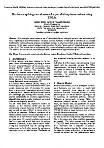
Fig. 2.
Problem decomposition based on output parallelism.
where
is the input vector of the th training pattern, is the desired output vector of the th training pattern, and is the number of training patterns. Suppose we divide the original problem into subproblems -dimensional output each of which has a space (4) is the desired output vector of the th training where pattern for the th subproblem, as shown in Fig. 2. Each subproblem is solved by growing and training a feedforward neural network (module). A collection of such modules is the overall solution of the original problem. In the following, we present why this method does work. Many different cost functions (also called error measures) can be used for network training. The most commonly used one is the sum of squared errors and its variations (5) is the actual output value of the th output unit for where is the desired output value of the the th training pattern and th output unit for the th training pattern. If we divide the output vector into sections, each of which output unit(s), then (5) can be transformed into contains
B. Task Decomposition The decomposition of a large-scale and complex problem into a set of smaller and simpler subproblems is the first step to implement modular neural network learning. Our approach is to split this complex problem with high-dimensional output space into a set of subproblems with low-dimensional output spaces. be the training set for a problem with -dimensional Let output space (3)
(6)
GUAN AND LI: PARALLEL GROWING AND TRAINING OF NEURAL NETWORKS
where , and . is independent of each other We can see and the only constraint among them is their sum should be small enough (acceptable). We can make each module’s error small enough to gurantee the overall error small enough. We can divide the original problem into subproblems. Each subproblem is composed of the whole input vector and a fraction of the output vector to produce the corresponding fraction of the output vector for the original problem. Obviously, the collection of modules (for subproblems) is equivalent to the nonmodular network. Furthermore, the hidden structures for the original problem’s output units are decoupled. This allows the hidden units in modular to act more as feature detectors output units than in a classic nonmodular network. for the Consequently, weight modification in each module is guided by only one portion of output units and learning is likely to be more efficient and the error to be smaller. Output parallelism to its extreme can be free from internal interference caused from output clash as each output is derived independently so that there is no way for the hidden units to receive contradictory signals from two or more output units. Output parallelism partitioning the output units into subsets can still reduce internal interference caused from output clash as each output subset is a portion of the original output units, which means any internal interference within the subset will be less likely and will be a subset of the internal interference in the original network. The internal interference from each subset combined will be less than the internal interference from the full set of original output units.
545
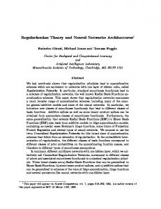
Fig. 3. Nonmodular and modular network architecture.
Fig. 4.
The parallel growing and training procedure.
C. Parallel Growing and Results Merging
D. Some Definitions and the Stopping Criteria for Growing and Training Modules
After problem decomposition, the original problem is divided into subproblems. Each subproblem is solved by growing and training a module. So the original neural network (nonmodular network) for the original problem is replaced by the modular network, as shown in Fig. 3. In the modular network architecture, each module can grow and be trained in parallel, in different processing elements. When we apply the modules for new input data, each module is responsible for calculating a fraction of the output and their results are merged to generate the final output for the given data. The procedure for parallel growing and training modules to solve the original problem is shown in Fig. 4. First, divide the original problem into subproblems. Then construct modules for the subproblems. The procedure for growing and training each module will be described in Section III-D. Last, merge the results of subproblems to form the solution for the original problem. In our method, communication overhead is very little since each module is constructed independently. Before learning, we need to deliver a copy of the training patterns for each module. However, during the learning process, no communication is needed among the modules. In the recall phase, to obtain the results for the incoming patterns, we only need to merge the collection of modules to form a modular network, as shown in Fig. 3(b).
As mentioned in Section II, Sections III-A–C, the reason why CBP is selected is that the implementation of CBP is simple and we do not need to switch between two different cost functions like in the CC algorithm. And we only need to backpropagate the output error through one and only one hidden layer. This way the CBP algorithm is computationally as efficient as the CC algorithm [8]. Although constructive learning algorithms have many advantages [1], [12], they are very sensitive to changes in the stopping criteria. If training is too short, the components of the network will not work well to generate good results. If training is too long, it costs much computation time and may result in overfitting and poor generalization. Referring to [13], [14], we adopted the method of early stopping using a validation set to prevent overfitting. The set of available patterns is divided into three sets: a training set is used to train the network, a validation set is used to evaluate the quality of the network during training and to measure overfitting, and a test set is used at the end of training to evaluate the resultant network. The size of the training, validation, and test set is 50%, 25%, and 25% of the problem’s total available patterns. used is the squared error percentage The error measure [13], derived from the normalization of the mean squared error
546
IEEE TRANSACTIONS ON NEURAL NETWORKS, VOL. 13, NO. 3, MAY 2002
to reduce the dependency on the number of coefficients in the problem representation and on the range of output values used (7) and are the maximum and minimum values of where output coefficients in the problem representation. is the average error per pattern of the network over is the training set, measured after epoch . The value the corresponding error on the validation set after epoch and is the corresponding is used by the stopping criterion. error on the test set; it is not known to the training algorithm but characterizes the quality of the network resulting from training. is defined to be the lowest validation set The value error obtained in epochs up to epoch : (8) The generalization loss [13] at epoch is defined as the relative increase of the validation error over the minimum so far (in percent) (9) A high generalization loss is one candidate reason to stop training because it directly indicates overfitting. To formalize the notion of training progress, a training strip of length [13] is defined to be a sequence of epochs numbered where is divisible by . The training progress measured after a training strip is
(10) It is used to measure how much larger the average training error is than the minimum training error during the training strip. During the process of growing and training individual modules, we adopted the following heuristic overall stopping criOR (Reduction of training set error due to teria: the last new hidden unit is less than 0.01% AND Validation set error increased due to the last new hidden unit). The first part means that the optimal validation set error is and the result has been acceptable. below the threshold The other part means the last insertion of a hidden unit resulted in hardly any progress. The criteria for adding a new hidden unit are as follows: At least 25 epochs reached for the current netOR Training progress work AND (Generalization loss 0.1). The first part means that the current network should be trained for at least a certain number of epochs before a new hidden unit is installed because the error curves may be turbulent at the beginning. The second part means that the current network has been overfitted or training has little progress. It is a bit unsatisfactory that all of these criteria are heuristic. However, as mentioned by Prechelt [7], there is no theory that would allow the derivation of criteria that are both efficient and effective.
IV. EXPERIMENTAL RESULTS AND ANALYSIS A. The Experiment Scheme Five benchmark problems, namely, the Building1, Flare1, Diabetes1, Glass1, and Vowel problem, are used to evaluate the effectiveness of parallel constructing neural networks based on output parallelism. The first four problems are all taken from the PROBEN1 benchmark collection [22] and the vowel problem is taken from University of California at Irvine (UCI) repository of machine learning databases. Building1 and Flare1 are two regression problems and the others are classification problems. We used the RPROP algorithm [20] to minimize the cost functions. In the set of experiments undertaken, each problem was conducted 20 runs. The RPROP algorithm used the fol, , , lowing parameters: , with initial weights from 0.25 0.25 randomly. In all experiments, the hidden units and output units is set to 0.1. When a all use sigmoid activation function and hidden unit needs to be added, eight candidates are trained and the best one is selected. All the experiments are simulated on a Pentium III–650 PC. The subproblems are solved sequentially and their CPU times expended are recorded, respectively. B. Results and Analysis Several issues are of particular importance: generalization accuracy, learning speed, and network complexity. As to generalization accuracy, for classification problems, we pay more attention to classification error than test error; for regression problems, we pay attention only to test error. It should be noted that each module might have different number of output units and the nonmodular network has more output units than a module. Therefore, the computational cost of one epoch can differ significantly among the modules and nonmodular network. Comparing the number of epochs solely will be misleading. So for learning speed, we place the emphasis on training time instead of epochs. As far as network complexity is concerned, the number of independent parameters (the number of weights and biases in the net) is more significant than the number of hidden units due to the same reason. 1) Building1: The Building1 problem predicts the energy consumption in a building. It tries to predict the hourly consumption of electrical energy, hot water, and cold water, based on the date, time of day, outside temperature, outside air humidity, solar radiation, and wind speed. It has 14 inputs, three outputs, and 4208 patterns. Building1 is divided into three subproblems and each has only one output unit. Each subproblem is solved by growing and training one module. From Table I, we can see that test error obtained by the modular network (0.483) is much smaller than that obtained by the nonmodular network (0.612). The maximum training time consumed for the three modules is 79.80 s, much less than that for the nonmodular network (122.50 s). To obtain this performance figure, a parallel computer is required with each processing element (PE) being a Pentium III–650 PC for each module. It is noted that the amount of time expended for merging the modules to form the modular network and delivering the test patterns for obtaining the overall solution is very little, about only 0.35 s (80.15 s–79.80 s). It is also noted that
GUAN AND LI: PARALLEL GROWING AND TRAINING OF NEURAL NETWORKS
TABLE I RESULTS FOR BUILDING1
547
TABLE II RESULTS FOR FLARE1
*Percentage of test error reduction by modular network (0.542) versus nonmodular network (0.555): 2.34%. *Percentage of test error reduction by modular network (0.483) versus nonmodular network (0.612): 21.8%. Note: 1. In the Problem column, “modular” stands for modular network, i.e., the collection of all the modules. It is the overall solution for the original problem based on output parallelism. “Nonmodular” stands for nonmodular network. It is the solution for the original problem using the conventional method. 2. “T.Time” stands for training time, the CPU time taken by growing and training each module or nonmodular network. For the modular network, “T. Time” equals to the maximum “T. Time” of the modules plus the time expended for merging the modules to form the modular network and delivering the test patterns to obtain the overall solution. 3. “Ind. Param.” stands for the number of independent parameters (the number of weights and biases in the net. 4. “Ete” stands for the test error and “C. Error” stands for classification error. For regression problems (Building 1 and Flare1), we consider test error only. 5. For the date, the first row is the average and the second row is its standard deviation.
the experiment results show that our approach improves generalization accuracy, regardless whether training time is saved or not (i.e., if there is no parallel computer to run our proposed method). As to network complexity, the maximum number of independent parameters among the three modules is 138 while the nonmodular network has 167 independent parameters. It is unfair to compare the total number of independent parameters of the modular network with that of the nonmodular network. As we anticipated that the former would usually be larger than the latter. However, each module has a distinctly different number of independent parameters, which explains why we should adopt a constructive learning algorithm instead of a predefined network architecture. 2) Flare1: Flare1 is a regression problem. It predicts solar flares by trying to guess the number of solar flares of small, medium, and large sizes that will happen during the next 24-hour period in a fixed active region of the Sun surface. Its input values describe previous flare activity and the type and history of the active region. Flare1 has 24 inputs, three outputs, and 1066 patterns. The Flare1 problem is divided into two subproblems. The first one (module 1) has one output unit and the second one (module 2) has two output units. From Table II, we can see the modular network spends only about half the training time of the nonmodular network. And the former obtains smaller test error as well. 3) Diabetes1: The Diabetes1 problem diagnoses diabetes of Pima Indians. It has eight inputs, two outputs, and 768 patterns.
TABLE III RESULTS FOR DIABETES1
*Percentage of test error reduction by modular network (16.047) versus nonmodular network (16.115): 0.42%. **Percentage of classification error reduction by modular network (23.359) versus nonmodular network (23.932): 2.39%.
All inputs are continuous. Its attributes are: number of times pregnant, plasma glucose concentration, diastolic blood pressure, triceps skin fold thickness, 2-h serum insulin, body mass index, diabetes pedigree function, and age. We divide the Diabetes1 problem into two subproblems each of which has one output unit. As shown in Table III, each module spends much less training time and has simpler network than the nonmodular network. The modular network obtained smaller classification error and test error also compared with the nonmodular network. 4) Glass1: This data set is used to classify glass types. The results of a chemical analysis of glass splinters (percentage of eight different constituent elements) plus the refractive index are used to classify a sample to be either float processed or nonfloat processed building windows, vehicle windows, containers, tableware, or head lamps. This task is motivated by forensic needs in criminal investigation. This data set consists of nine inputs, six outputs, and 214 patterns. The Glass1 problem is divided into two subproblems each of which has three output units. The classification error is significantly reduced from 40.236% to 34.906% as we use the modular network instead of the nonmodular network.
548
IEEE TRANSACTIONS ON NEURAL NETWORKS, VOL. 13, NO. 3, MAY 2002
TABLE IV RESULTS FOR GLASS1
TABLE V RESULTS FOR VOWEL
*Percentage of test error reduction by modular network (9.233) versus nonmodular network (9.881): 6.56%. **Percentage of classification error reduction by modular network (34.906) versus nonmodular network (40.236): 13.25%.
5) Vowel: The data set used in this example were obtained from the University of California at Irvine (UCI) repository of machine learning databases. The input patterns are ten element real vectors representing vowel sounds which belong to one of 11 classes. It has 990 patterns in total. The patterns were normalized and scaled so that each components lies within . We divide the Vowel problem into 11 subproblems and each has one output unit. From Table V, we can see that training time for the modular network is 184.63 s, less than one third of that for the nonmodular network, 622.55 s. At the same time, the classification error obtained by the modular network is 24.355%, much smaller than that of the nonmodular network, 34.737%. As a contrast, the classification error obtained in [25] is 44.7%. From the experiments, we can see that our method is especially good for those problems that have a large number of output units, e.g., the Vowel problem and the Glass1 problem. Their classification error and test error are reduced dramatically based on output parallelism. This is because conflicting signals from different output units retard learning in a nonmodular network. However, in modular network, the hidden structures for the original problem’s output units are decoupled and consequently the internal interferences reduce. Therefore, weight modification in each module is guided by only one portion of output units and learning is likely to be more efficient and the error to be smaller. is set to 0.1. For In our experiments presented above, some problems (validation set errors obtained by some individual modules are below 0.1), we can actually set a smaller . The results obtained when is set to 0.01 for Building1 and Glass1 are displayed in the Appendix. From the results, we can see that their test errors and classification errors are reduced further compared to the results in Tables I and IV. Note that the test errors and classification errors from the nonmodular network remain the same for these two problems. The cost of doing this is that some modules will have a few more independent parameters than the previous results.
*Percentage of test error reduction by modular network (3.610) versus nonmodular network (4.557): 20.78%. **Percentage of classification error reduction by modular network (24.355) versus nonmodular network (34.737): 28.89%.
V. CONCLUSION This paper presents an approach to grow and train neural networks based on output parallelism. Feasibility of output parallelism is analyzed and proved by (6). A problem can be divided into several subproblems, each of which is composed of the whole input vector and a fraction of the output vector. Each module (for one subproblem) thereby is responsible for producing a fraction of the output vector of the original problem. Such modules can be grown and trained in parallel. Based on output parallelism, a complex problem can be divided into several simpler subproblems as chosen, and internal interference is greatly reduced. This is because the hidden structure for the original problem’s output units are decoupled. Efficient and effective learning is consequently achieved. It should be mentioned that problems that have only one output unit cannot be decomposed using our method. And as we can see from the experiments, our method is especially good for the problems that have a large number of output units.
GUAN AND LI: PARALLEL GROWING AND TRAINING OF NEURAL NETWORKS
TABLE VI RESULTS FOR BUILDING1 (E
IS
SET TO 0.01)
*Percentage of test error reduction by modular network (0.481) versus nonmodular network (0.612): 21.41%.
From the results obtained by our experiments, we can summarize the advantages of output parallelism as follows: 1) A problem can be decomposed into a set of subproblems as chosen without any prior knowledge concerning the decomposition of the problem. 2) In a nonmodular network, conflicting signals from different output units retard learning. Modular learning based on output parallelism is likely to be more efficient and effective, since weight modification is guided by only one portion of output units. 3) Individual modules in a modular network are simpler than the nonmodular network, and a smaller error threshold are likely to be achieved. 4) Although the total number of independent parameters in all the modules usually exceeds that in the nonmodular network, the modular approach yields faster convergence and better generalization accuracy. 5) Since each subproblem can be learned independently, different constructive learning algorithms and different network structures can be used to learn each subproblem. 6) Since each subproblem can be learned independently, they can be learned and recalled in parallel on multiple processing elements.
VI. FUTURE WORK In our experiments, the problems are decomposed into a number of subproblems and better generalization accuracy and less network complexity is achieved. As we have seen that different subproblems have different complexities and generally require different training time. In practice, different processing elements may have different computation power. An interesting problem is how to predict subproblem’s complexity and schedule a balanced computation load for each processing element in order to minimize idle time. This will be further studied in our future work.
549
TABLE VII RESULTS FOR GLASS1 (E IS SET TO 0.01)
*Percentage of test error reduction by modular network (9.177) versus nonmodular network (9.881): 7.12%. **Percentage of classification error reduction by modular network (34.528) versus nonmodular network (40.236): 14.19%.
APPENDIX In this section, we present the results obtained when is set to 0.01 for Building1 and Glass1 problem (see Tables VI and VII). ACKNOWLEDGMENT The authors thank the reviewers for their valuable comments. REFERENCES [1] A. Blum and R. L. Rivest, “Training a 3-node neural network is NP-complete,” Neural Networks, vol. 5, no. 1, pp. 117–128, 1992. [2] E. B. Baum and D. Haussler, “What size net gives valid generalization?,” Neural Comput., vol. 1, no. 1, pp. 151–160, 1989. [3] R. Reed, “Pruning algorithm—A survey,” IEEE Trans. Neural Networks, vol. 4, pp. 740–747, 1993. [4] T. Poggio and F. Girosi, “Regularization algorithms for leaning that are equivalent to multi-layer networks,” Science, vol. 247, pp. 978–982, 1990. [5] T. Y. Kwok and D. Y. Yeung, “Objective functions for training new hidden units in constructive neural networks,” IEEE Trans. Neural Networks, vol. 8, pp. 1131–1148, Sept. 1997. [6] T. Ash, “Dynamic node creation in backpropagation networks,” Connection Sci., vol. 1, no. 4, pp. 365–375, 1989. [7] L. Prechelt, “Investigation of the CasCor family of learning algorithms,” Neural Networks, vol. 10, no. 5, pp. 885–896, 1997. [8] S. E. Fahlman and C. Lebiere, “The cascade-correlation learning architecture,” in Advances in Neural Information Processing systems II, D. S. Touretzky, G. Hinton, and T. Sejnowski, Eds. San Mateo, CA: Morgan Kaufmann, 1990, pp. 524–532. [9] D. Y. Yeung, “A neural network approach to constructive induction,” in Proc. 8th Int. Workshop Machine Learning, Evanston, IL, 1991. [10] M. Lehtokangas, “Modeling with constructive backpropagation,” Neural Networks, vol. 12, pp. 707–716, 1999. [11] S. Sjogaard, “Generalization in cascade-correlation networks,” in Proc. IEEE Signal Processing Workshop, 1992, pp. 59–68. [12] J. Yang and V. Honavar, “Experiments With Cascade-Correlation Algorithm,” Dept. Comput. Sci., Iowa State Univ., 91-16, 1991. [13] C. S. Squires and J. W. Shavlik, “Experimental analysis of aspects of the cascade-correlation learning architecture,” in Machine Learning Research Group Working Paper 91-1: Comput. Sci. Dept., Univ. Wisconsin, Madison, 1991. [14] G. Auda, M. Kamel, and H. Raafat, “Modular neural network architectures for classification,” in Proc. IEEE Int. Conf. Neural Networks, vol. 2, 1996, pp. 1279–1284. [15] R. A. Jacobs, M. I. Jordan, M. I. Nowlan, and G. E. Hinton, “Adaptive mixtures of local experts,” Neural Comput., vol. 3, no. 1, pp. 79–87, 1991.
550
[16] P. Liang, “Problem decomposition and subgoaling in artificial neural networks,” in Proc. IEEE Int. Conf. Syst., Man, Cybern., Los Angeles, CA, 1990, pp. 178–181. [17] S. G. Romaniuk and L. O. Hall, “Divide and conquer neural networks,” Neural Networks, vol. 6, pp. 1105–1116, 1993. [18] A. J. C. Sharkey, “Modularity, combining and artificial neural nets,” Connection Sci., vol. 9, no. 1, pp. 3–10, 1997. [19] D. E. Rumelhart, G. E. Hinton, and R. J. Williams, “Learning internal representations by error propagation,” in Parallel Distributed Processing: Explanations in the Microstructure of Cognition, D. E. Rumelhart and J. L. McClell, Eds. Cambridge, MA: MIT Press, 1986, vol. 1, Foundation, pp. 318–362. [20] M. Riedmiller and H. Braun, “A direct adaptive method for faster backpropagation learning: The RPROP algorithm,” in Proc. IEEE Int. Conf. Neural Networks, 1993, pp. 586–591. [21] J. Torresen and O. Landsvek, “A review of parallel implementations of backpropagation neural networks,” in Parallel Architectures for Artificial Neural Networks: Paradigms and Implementations, N. Sundararajan and P. Saratchandran, Eds. Los Alamitos, CA: IEEE Comput. Soc. Press, 1998, pp. 25–63. [22] L. Prechelt, “PROBEN1: A set of Neural Network Benchmark Problems and Benchmarking Rules,” Dept. Informatics, Univ. Karlsruhe, Karlsruhe, Germany, 21/94, 1994. [23] B. L. Lu and M. Ito, “Task decomposition and module combination based on class relations: A modular neural network for pattern classification,” IEEE Trans. Neural Networks, vol. 10, pp. 1244–1256, Sept. 1999. [24] R. E. Jenkins and B. P. Yuhas, “A simplified neural network solution through problem decomposition: The case of the truck backer-upper,” IEEE Trans. Neural Networks, vol. 4, pp. 718–720, July 1993. [25] R. Anand, K. Mehrotra, C. K. Mohan, and S. Ranka, “Efficient classification for multiclass problems using modular neural networks,” IEEE Trans. Neural Networks, vol. 6, pp. 117–124, Jan. 1995. [26] K. Chen, L. Yang, X. Yu, and H. Chin, “A self-generating modular neural network architecture for supervised learning,” Neurocomput., vol. 16, pp. 33–38, 1997. [27] P. Gallinari, “Modular neural net systems, training of,” in The Handbook of Brain Theory and Neural Networks, M. A. Arbib, Ed. Cambridge, MA: MIT Press, 1995, pp. 582–585. [28] S. Kumar and J. Ghosh, “GAMLS: A generalized framework for associative modular learning systems,” in Proc. Applicat. Sci. Comput. Intell. II, Orlando, FL, 1999, pp. 24–34. [29] V. Petridis and A. Kehagias, Predictive Modular Neural Network: Applications to Time Series. Boston, MA: Kluwer, 1998.
IEEE TRANSACTIONS ON NEURAL NETWORKS, VOL. 13, NO. 3, MAY 2002
[30] L. Su and S.-U. Guan, “Two-dimensional extensions of cascade correlation networks,” in Proc. 4th Int. Conf./Exhibition High Performance Comput. Asia-Pacific Region, vol. 1, 2000, pp. 138–141. [31] S.-U. Guan and S. Li, “An approach to parallel growing and training of neural networks,” in Proc. 2000 IEEE Int. Symp. Intell. Signal Processing Commun. Syst. (ISPACS2000), Honolulu, HI. [32] B. L. Lu, H. Kita, and Y. Nishikawa, “A multisieving neural-network architecture that decomposes learning tasks automatically,” in Proc. IEEE Conf. Neural Networks, Orlando, FL, 1994, pp. 1319–1324. [33] M. I. Jordan and R. A. Jacobs, “Hierarchical mixtures of experts and EM algorithm,” Neural Comput., vol. 6, no. 2, pp. 181–214, 1994.
Sheng-Uei Guan received the M.Sc. and Ph.D. degrees from the University of North Carolina, Chapel Hill. He is currently an Associate Professor of the Electrical and Computer Engineering Department at National University of Singapore, Singapore. He has worked in a prestigious R&D organization for several years, serving as a Design Engineer, Project Leader, and Manager. He has also served as a Member on the R.O.C. Information and Communication National Standard Draft Committee. After leaving the industry, he joined Yuan-Ze University in Taiwan for three and half years. He served as Deputy Director for the Computing Center, and also as the Chairman for the Department of Information and Communication Technology. Later, he joined the Department of Computer Science and Computer Engineering, La Trobe University, Melbourne, Australia, where he helped to create a new multimedia systems stream.
Shanchun Li received the B.Eng. and M.Eng. degrees in mechanical engineering from Zhejiang University, P.R. China, in 1996 and 1999, respectively. He received the M.Eng. degree in computer engineering from National University of Singapore, Singapore, in 2001. He is now with Fuji Xerox Asia Pacific Pte Ltd.