Performance Visualization for Large-Scale Computing Systems: A ...

Performance Visualization for Large-Scale Computing Systems: A Literature Review Qin Gao1, Xuhui Zhang1, Pei-Luen Patrick Rau1, Anthony A. Maciejewski2, Howard Jay Siegel2,3 1

Department of Industrial Engineering, Tsinghua University, Beijing 100084, P. R. China 2 Electrical and Computer Engineering Department, 3Computer Science Department Colorado State University, Fort Collins, CO 80523-1373 USA {gaoqin, xuhuizhang,rpl}@tsinghua.edu.cn, {aam, hj}@colostate.edu

Abstract. Recently the need for extreme scale computing solutions presents demands for powerful and easy to use performance visualization tools. This paper presents a review of existing research on performance visualization for large-scale systems. A general approach to performance visualization is introduced in relation to performance analysis, and issues that need to be addressed throughout the performance visualization process are summarized. Then visualization techniques from 21 performance visualization systems are reviewed and discussed, with the hope of shedding light on the design of visualization tools for ultra-large systems. Keywords: performance visualization, performance monitoring, information visualization

1

Introduction

Performance visualization is the use of graphical display techniques for the visual analysis of performance data. The process can be abstracted as a mapping from system behaviors to visual representations [1, 2]. By augmenting cognition with the human visual system’s highly tuned ability to see patterns and trends, performance visualization tools are expected to aid comprehension of the dynamics, intricacies, and properties of program execution [3, 4]. Recently the need for extreme scale computing solutions [5] presents new challenges for the design and development of performance visualization tools. It is expected that next-generation supercomputers (so-called exascale computers) will be more than 1000 times faster than the current petascale systems. Such an increase in performance is associated with an increase in the level of parallelism, the heterogeneity of computing resources, and the complexity of interactions among these resources [6, 7]. Monitoring program run-time behaviors to tune performance in real-time is indispensible to realizing the potential of such systems, but the immense volume and complexity of the performance data presents a major challenge for human perception and cognition. Powerful and easy to use performance visualization is important to solving this problem.

This paper presents a review of performance visualization tools for large-scale systems. The goal is not to exhaustively enumerate visualization systems, but to describe issues that need to be addressed throughout the performance visualization process, with the hope of shedding light on design of visualization tools for ultra-scale systems. In Section 2, a general approach to performance visualization is introduced, and issues related to each phase are discussed. Section 3 presents a review of visualization techniques from 21 performance visualization systems. The framework of information visualization by Card [3] is adopted to classify and analyze these techniques. Implications for future research are presented in Section 4.

2

Approach to Performance Visualization

According to literature on performance analysis and visualization [1, 3, 4, 11, 12], the process of performance visualization generally consists of four major steps: instrumentation (enabling access to performance data to be measured), measurement (recording selected data during the run-time of the program), data analysis (analyzing data for performance visualization), and visualization (mapping performance characteristics to proper visual representations and interactions). A major challenge for instrumenting large systems is to decide what to be instrumented among a huge amount of data of different levels from numerous heterogeneous sources. The data to be collected should reflect application performance as closely as possible while minimizing perturbation of that behavior as much as possible (trade-off between fidelity and perturbation) [12]. The instrumentation may reside in hardware or in software. Hardware instrumentation involves a monitoring system collecting performance data, and generally incurs less performance degradation than software instrumentation. But the portability of this approach is low due to the requirement of dedicated monitoring hardware. Software instrumentation involves inserting small pieces of code, often referred to as sensors, in the operation system, the run-time environment, or the application program. This process can easily become tedious and time-consuming for large systems, and automation is desired to reduce the effort from application developers. During the execution of applications, performance data can be measured by tracing (recording individual events and associated data) or by profiling (recording summary trends and statistics). Tracing provides more execution information, and is necessary for tools aiming to visualize detailed program run-time behaviors, such as [13-15]. Profiling collects only summary statistics, usually with hardware counters. This approach imposes less perturbation than tracing, but sacrifices fidelity. Tools using profiling, such as SvPablo [16], often allow data collection for large systems with long execution times. The recording action can be triggered either under specific conditions (event-driven, also called tracing by [11]) or periodically (sampling). Some tools support both approaches, such as [17]. The collected data can be analyzed and visualized during execution, as with Paradyn [18] and Virtue [13], or saved to a trace file for post mortem analysis, as with ParaGraph [2] and SvPablo [16]. For distributed applications in which resource availability changes dynamically, real-time measurement and visualization is necessary for effective performance tuning [13].

After a stream of performance data has been collected, data analysis will be performed to calculate various metrics required for performance evaluation and visualization, including microscopic metrics of individual components (e.g., processor state and execution rate) and macroscopic metrics of overall performance (e.g., concurrency, load balance). To extract useful information from a morass of performance data, data reduction methods (e.g., summation, averaging, extrema finding) are often used. Some systems make use of multivariate statistical analysis techniques, such as correlation, clustering, and multidimensional scaling, in search of recognizable relationships among related variables. In addition, a number of performance analysis systems developed application-specific analysis techniques for recognizing high-level program behaviors [19], pointing out causes of poor performance, generating scalability trends [9], and other application-specific purposes. In the visualization phase, extracted performance metrics and relationships are mapped into selected visual structures, which are then integrated and transformed to form visualization views. Despite the seemingly hopeless variability of visual forms that could result, Card suggested that only a limited number of visual components are involved in information visualization due to various constraints to which such visualizations are subjected [3]. The basic visual components include the spatial substrate that defines the space, marks appearing in the space, connections and enclosures for linking and enveloping, retinal properties (graphic properties to which the retina of human eyes are sensitive independent of position, such as color, size, shape, texture, and orientation) overlaying other components, and temporal encoding for tracking changes of graphic properties.

3

Review of Visualization Techniques

3.1

Classification of Visualization Techniques

In this section, we will review visualization techniques from 21 performance visualization systems. These techniques can be classified into the categories of the information visualization taxonomy proposed by Card [3], as shown in Table 1. 3.2

Simple Visual Structures

Statistical charts with one or two variables. The simplest form of performance visualization is to use common statistical charts and diagrams, such as bar charts, pie charts, kiviat diagrams, and matrix views, to show summary statistics of computation, utilization, and communication metrics. These simple charts could be powerful, because they provide an overview of important performance metrics and enable quick identification of major problems, such as overload and imbalance. They are used widely in performance visualization systems, such as ParaGraph [2] and AIMS [9].

Table 1. Classification of performance visualization techniques. Category Simple visual structures

Performance Visualization Techniques Pie charts, distribution, box plots, kiviat diagrams Timeline views

Information typologies

Information landscape Trees & networks Composed visual structures Interactive visual structure

Focus + context visual structures

Single-axis composition Double-axis composition Case composition Interaction through controls (data input, data transformation, visual mapping definition, view operations) Interaction through images (magnifying lens, cascading displays, linking and brushing, direct manipulation of views and objects) Macro-micro composite view

Example applications and studies ParaGraph [2], PET [20], SvPablo [16], VAMPIR [21], Devise [22], AIMS [9] Paje [23], AIMS [9], Devise [22], AerialVision [24], Paraver [25], SIEVE [14], Virtue [13], utilization and algorithm timeline views in [17] SHMAP [26], Vista [4], Voyeur [27], processor and network port display in [28], hierarchical display in [12] Triva [29], Cichild [30] Paradyn [18], Cone Trees [31], Virtue [13], [32] AIMS [9], Vista [4] Devise [22], AerialVision [24] Triva [29] Paje[23], data input, filtering, and view manipulation in [28] and [32] Virtue [13], Cone Trees [31], Devise [22], direct manipulation of the 3D cone and virtual threads in [32] Microscopic profile in [4], PC-Histogram in [24]

Timeline views. Use of timeline views in performance visualization systems can be classified into the following groups:

(a)

(b)

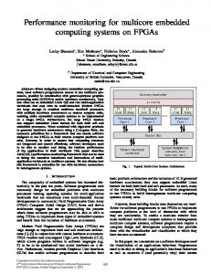
Fig. 1. Time views of program execution and communications. (a) Pajé: visualization of program execution and communication [33] (b)Virtue: time-tunnel display [13]

 Describing run-time behaviors and communication paths Fig. 1(a) shows a typical visualization of program behaviors and communications. Time is mapped to the horizontal axis, and horizontal bars ranked along the vertical axis represent system components being analyzed, such as processors, tasks, and threads. Communications between the components are represented by arrows between bars. Colors are used to indicate the component status or the type of activities. The time lines can also be organized non-linearly, as in the time-tunnel display shown in Fig. 1(b). Other performance data can be added by using extra retinal features, such as textures and shapes [9, 15, 20]. A problem of such timeline views is that they scale poorly when system sizes increase. One way to mitigate the problem is to use more

concise displays, such as the space-time diagram from ParaGraph [2]. Other methods to improve the scalability of such timeline views are discussed in [33, 34].  Showing the evolution of performance statistics over time This type of visualization plots summary performance metrics versus time, often using line plots (top plot in Fig. 2) or bar charts. It is often used to plot several different metrics or the same metrics related to different system components (e.g., different nodes, processes) versus time on a single view so they may be compared. Multiple metrics can be visualized as multiple line plots (middle plot in Fig. 2), stacked bar charts, or intensity plots (bottom plot in Fig. 2).

Fig. 2. Time views of utilization/computation/communication summaries of AerialVision, with the top plot showing global IPC, the middle plot showing the average memory queue occupancy for each DRAM channel, and the bottom plot showing the same data as the middle plot but using intensity plot (the darker the color, the higher memory queue occupancy) [24]

 (a)

(b)

Fig. 3. Timeline views to facilitate source code level analysis. (a) AerialVision: PC-Histogram [24]. (b) SIEVE: Contour-plot [14].

 Facilitating source code level analysis Fig. 3(a) presents a visualization of source code execution over time from AerialVision [24]. Program code is laid out in ascending source line number along the vertical axis. The time period in which the portion of a program is fetched in the pipelines is colored, where the intensity represents the number of threads fetching the portion of the program at the given time point. With this visualization, it is easy to identify the instructions that cause threads to become delayed, which are indicated by horizontal lines on the plot. Fig. 3(b) shows another visualization of source code execution from SIEVE [14], which displays calling to a specific function by processors as contours. Information typography. Information typography is an essentially 2D scatterplot, with the two spatial dimensions partly defined by external structures, and retinal variables (e.g., colors, shapes) used as an overlay to add more information. Being able

to combine performance data with physical topology, this visualization is especially useful for geographically distributed applications and systems with complex interconnection topologies. Fig. 4(a) shows an information typology of a large-scale cluster [28]. Network switches are arranged according to system interconnection topology. Colors are used to indicate the computational job and associated performance data, and thick line segments are used to show routing information once the route source and destination have been selected. Information typography can also be used to integrate logical architectures, as in [12].

(a)

(b)

Fig. 4. Information typography and information landscape. (a) Port display on network typology [28]. (b) Triva: information landscape based on resource hierarchy.

Information landscape. Information landscapes differ from information topographies in that they have one variable extruded into the third spatial dimension. Fig. 4(b) presents an information landscape from Triva [29]. The time axis is mapped to the vertical axis. Each vertical bar represents the progression of a process, and different states along the time axis are represented by different colors. These processes are put on top of a visual base (shown as colored rectangles), which is organized as a treemap [35] of the resource hierarchy.

(a)

(b)

(c)

Fig. 5. Trees and networks. (a) Paradyn: Performance Consultant, showing a search hierarchy [18]. (b) Cone Trees: 3D visualization of tree structures [31]. (c) Virtue: Geographic network display [13].

Trees and networks. Trees and networks differ from other visual structures in the use of explicitly drawn linkages for spatial positioning [3]. Trees are used to describe hierarchical information structures like resource hierarchies [36, 37]. AIMS uses trees to illustrate the dependency between hypotheses in a search for performance bottlenecks, as shown Fig. 5(a). A significant limitation of trees is that the nodes expand exponentially as a function of depth, which leads to an extreme aspect ratio for large trees. A possible solution is Cone Trees [31] (Fig. 5 (b)), which utilize 3D

interactive visualization to make effective use of screen space and enable visualization of whole tree structures. Networks are useful for describing network connections, communication traffic, and relationships or communications among program entities. Fig. 5(c) shows a geographic network display from Virtue [13]. Vertices are placed on the global map according to the geographic distribution of resource sites, and retinal properties of vertices and edges are used to encode information like latency and bandwidth. 3.3 Composed Structures A composed structure is a synthesis of two or more simple structures into a single compound view, with the aim to understand the relationship among variables or to provide a global image. There are several ways to produce a composed structure:  Single-axis composition: multiple graphs sharing a single axis are aligned to produce a new view. Time, process, and resource identifiers are often used as the common axis. A special case of single-axis composition is small multiples [10], which presents a series of images showing the same combination of variables indexed by changes in another variable, and the information slices can be played as successive frames like a movie, or positioned to a third spatial dimension, as in [4].  Double-axis composition: multiple graphs sharing two axes are plotted on a single graph. Fig. 6 shows an example from Devise [22]. The five small scatter plots show message bytes sent versus message bytes received for five processes, and the left plot is a composite of all of them, using different colors for encoding processes.  Case composition: two different graphs describing the same cases can be fused into a single diagram by having a single mark for each case. Triva’s information landscape shown in Fig. 6(b) is essentially a composition of a treemap of resource hierarchy and a communication timeline view.

Fig. 6. Message traffic plot from Devise [22] .

3.4

Interactive Visual Structures

Performance visualization systems provide a variety of user interactions to let the user select the portion of information they want to study and customize the way the information is presented, such as selecting alternative views, changing observation perspectives, zooming between different levels of detail, and manipulating other display parameters to acquire information they need to understand concurrent application behaviors. Interactive visual structures can be further divided into [1]:

 Direct interaction through the visualization: users manipulate the image directly to change the view. The simplest form of direct interaction is clicking a visual component to bring forward a more detailed view. An extension of this interaction is magnifying lens, which can be moved across the display and reveal hidden details when being hold over an object [13]. Other direct manipulations include panning the display by dragging, selecting visual objects, and re-positioning them. To make such direct manipulations more “natural” and immersive, Virtue [13] utilized virtual reality technologies to enable users to control the visualizations by gestures or direct manipulation of 3D sliders. For information at different grain sizes, cascading displays are often used, as in the case of Cone Tree shown inFig. 5 (b). When two or more representations of the same data are presented together, the coordination between windows can be controlled through interactive visual structures, such as the graphical cursor in Devise [22].  Indirect interaction though controls: users manipulate visualizations indirectly through predefined controls on the user interface. Interactions with the underlying computation, such as data-related controls (e.g., data input, filtering, grouping, and other transformation) and definitions of visual mappings (e.g., definition of colors, forms, and mapping relationships), are often carried out in this way. Common controls for view configurations include scroll-bars, zoom in/out buttons, sliders or input field for dynamic queries [28], and radio buttons for selecting specific characteristics to show [15]. 3.5

Focus + Context Abstractions

Focus + context abstractions refer to visualizations whose mappings are modified by the computer, not by the users themselves, according to its model of the users’ level of interest. In our survey, we found the use of such abstractions in performance visualization systems to be very limited. The only type being used is macro-micro composition [4, 24], in which both global picture and local details are provided, and detailed information accumulates into larger coherent structures. Focus + context abstractions are effective in combining overview and detail information in a single dynamic display. The scarcity of this type of visualization among performance visualization techniques may indicate directions for future performance visualization technique design.

4

Future work

In this paper, we summarized issues that need to be addressed throughout the process of performance visualization and reviewed visualization techniques from 21 performance visualization systems using Card’s framework of information visualization. These systems are built for monitoring and analyzing performance of parallel and distributed systems. Experiences gained and lessons learned from them could provide insight for the design of performance visualization tools for exascale computing systems, though there are new challenges. One major challenge is the huge

size of exascale systems, which requires good scalability of performance visualization techniques. On the one hand, data abstraction methods that are used widely in scientific visualization may be adapted to performance visualization. On the other hand, visualizations based on focus + context abstractions may help to combine highlevel context and low-level details in a more effective way. Other challenges are ergonomics and usability issues related to performance visualization for super-scale systems. Without considering the limitations of human sensory and cognition capabilities, the complexity of performance visualizations may easily exceed them. These issues should be addressed by future research in the field of visualization. Acknowledgment. This research was supported in part by the US National Science Foundation Grant number 0905399, and the CSU Abell Endowment.

References 1. Roman, G.C., Cox, K.C.: A taxonomy of program visualization systems. Computer. 26, 11-24 (2002). 2. Heath, M., Etheridge, J.: Visualizing the performance of parallel programs. IEEE Software. 8, 29--39 (1991). 3. Card, S.: Information visualization. In: The human-computer interaction handbook: Fundamentals, evolving technologies and emerging applications. pp. 509--543 (2002). 4. Rover, D.T.: A performance visualization paradigm for data parallel computing. TwentyFifth Hawaii Int. Conf. System Sciences. pp. 149--160 (2002). 5. Simon, H., Zacharia, H., Steven, R.: Modeling and simulation at the exascale for energy and the environment. Technical report, Department of Energy (2007). 6. Shestak, V., Smith, J., Maciejewski, A. A., Siegel, H.J.: Stochastic robustness metric and its use for static resource allocations. Journal of Parallel and Distributed Computing. 68, 1157-1173 (2008). 7. Ali, S., Maciejewski, A. A., Siegel, H. J., Kim, J. K.: Measuring the robustness of a resource allocation. IEEE Trans. Parallel and Distributed Systems. 15, 630--641 (2004). 8. Miller, B.P.: What to draw? When to draw? An essay on parallel program visualization. Journal of Parallel and Distributed Computing. 18, 265--269 (1993). 9. Yan, J., Sarukkai, S., Mehra, P.: Performance measurement, visualization and modeling of parallel and distributed programs using the AIMS toolkit. Software Practice & Experience. 25, 429--461 (1995). 10.Tufte, E.R.: Envisioning Information. Graphics Press, Cheshire, CT (1990). 11.Kraemer, E., Stasko, J.T.: The visualization of parallel systems: An overview. Journal of Parallel and Distributed Computing. 18, 105--117 (1993). 12.Koehler, S., Curreri, J., George, A.D.: Performance analysis challenges and framework for high-performance reconfigurable computing. Parallel Computing. 34, 217--230 (2008). 13.Shaffer, E., Reed, D.A., Whitmore, S., Schaeffer, B.: Virtue: Performance visualization of parallel and distributed applications. Computer. 32, 44--51 (2002). 14.Sarukkai, S.R., Gannon, D.: Parallel program visualization using SIEVE.1. 6th Int. Conf. Supercomputing - ICS '92. pp. 157--166 (1992). 15.De Kergommeaux, J.C., Stein, B., Bernard, P.E.: Pajé, an interactive visualization tool for tuning multi-threaded parallel applications. Parallel Computing. 26, 1253--1274 (2000). 16.De Rose, L., Reed, D.: SvPablo: A multi-language architecture-independent performance analysis system. 1999 Int. Conf. Parallel Processing. pp. 311--318 (1999).

17.Alexandrov, A., Armstrong, D., Rajic, H., Voss, M., Hayes, D.: High-level performance modeling of task-based algorithms. Int. Symp. Performance Analysis of Systems and Software (ISPASS). pp. 184--193 (2010). 18.Miller, B.P., Callaghan, M.D., Cargille, J.M., Hollingsworth, J.K., Irvin, R.B., Karavanic, K.L., Kunchithapadam, K., Newhall, T.: The Paradyn parallel performance measurement tool. Computer. 28, 37--46 (1995). 19.Bates, P.C.: Debugging heterogeneous distributed systems using event-based models of behavior. ACM Trans. Computer Systems (TOCS). 13, 1--31 (1995). 20.Garcia, J., Entrialgo, J., Garcia, D.F., Diaz, J.L., Suarez, F.J.: PET, a software monitoring toolkit for performance analysis of parallel embedded applications. Journal of Systems Architecture. 48, 221--235 (2003). 21.Nagel, W.E., Arnold, A., Weber, M., Nagel, W.E., Arnold, A., Weber, M., Solchenbach, K.: VAMPIR: Visualization and Analysis of MPI Resources. Supercomputer. 12, 69--80 (1996). 22.Karavanic, K.L., Myllymaki, J., Livny, M., Miller, B.P.: Integrated visualization of parallel program performance data. Parallel Computing. 23, 181--198 (1997). 23.De Kergommeaux, C., Stein, B.D.O.: Flexible performance visualization of parallel and distributed applications. Future Generation Computer Systems. 19, 735--747 (2003). 24.Ariel, A., Fung, W.W., Turner, A.E., Aamodt, T.M.: Visualizing complex dynamics in many-core accelerator architectures. Int. Symp. Performance Analysis of Systems and Software (ISPASS). pp. 164--174 (2010). 25.Pillet, V., Labarta, J., Cortes, T., Girona, S.: Paraver: A tool to visualize and analyze parallel code. Transputer and Occam Developments, WOTUG-18. pp. 17--31 (1995). 26.Dongarra, J., Brewer, O., Kohl, J.A., Fineberg, S.: A tool to aid in the design, implementation, and understanding of matrix algorithms for parallel processors. Journal of Parallel and Distributed Computing. 9, 185--202 (1990). 27.Socha, D., Bailey, M.L., Notkin, D.: Voyeur: Graphical views of parallel programs. 1988 ACM SIGPLAN and SIGOPS Workshop on Parallel and Distributed Debugging - PADD '88. pp. 206--215 (1988). 28.Haynes, R., Crossno, P., Russell, E.: A visualization tool for analyzing cluster performance data. 2001 IEEE Int. Conf. Cluster Computing (CLUSTER'01). pp. 295--302 (2001). 29.Schnorr, L.M., Huard, G., Navaux, P.O.: Triva: Interactive 3D visualization for performance analysis of parallel applications. Future Generation Computer Systems. 26, 348--358 (2010). 30.Brown, J.A., McGregor, A.J., Braun, H.W.: Network performance visualization: Insight through animation. Passive and Active Measurement Workshop. pp. 33--41 (2002). 31.Robertson, G.G., Mackinlay, J.D., Card, S.K.: Cone Trees: Animated 3D visualizations of hierarchical information. SIGCHI Conf. Human Factors in Computing Systems: Reaching Through Technology, pp. 189--194 (1991). 32.Kim, Y.J., Lim, J.S., Jun, Y.K.: Scalable thread visualization for debugging data races in OpenMP programs. 2nd Int. Conf. Advances in Grid and Pervasive Computing. pp. 310-321 (2007). 33.De Kergommeaux, J., De Oliveira Stein, B.: Pajé: an extensible environment for visualizing multi-threaded programs executions. 6th Int. Euro-Par Conf. Parallel Processing. pp. 133-140 (2000). 34.Knüpfer, A., Voigt, B., Nagel, W., Mix, H.: Visualization of repetitive patterns in event traces. Workshop State-of-the-Art in Scientific & Parallel Computing. pp. 430--439 (2007). 35.Johnson, B., Shneiderman, B.: Tree-Maps: A space-filling approach to the visualization of hierarchical information structures. 2nd Conf. Visualization '91. pp. 284--291 (1991). 36.Heisig, S.: Treemaps for workload visualization. IEEE Computer Graphics and Applications. 23, 60--67 (2003). 37.Goldberg, J.H., Helfman, J.I.: Enterprise network monitoring using treemaps. 49th Annual Meeting of the Human Factors and Ergonomics Society. pp. 671--675 (2005).