Phoneme representation and classification in primary auditory cortex

Phoneme representation and classification in primary auditory cortex Nima Mesgarani, Stephen V. David, Jonathan B. Fritz, and Shihab A. Shammaa兲 Electrical and Computer Engineering & Institute for Systems Research, University of Maryland, College Park, Maryland 20742

共Received 5 June 2007; revised 15 October 2007; accepted 30 October 2007; corrected 20 March 2008兲 A controversial issue in neurolinguistics is whether basic neural auditory representations found in many animals can account for human perception of speech. This question was addressed by examining how a population of neurons in the primary auditory cortex 共A1兲 of the naïve awake ferret encodes phonemes and whether this representation could account for the human ability to discriminate them. When neural responses were characterized and ordered by spectral tuning and dynamics, perceptually significant features including formant patterns in vowels and place and manner of articulation in consonants, were readily visualized by activity in distinct neural subpopulations. Furthermore, these responses faithfully encoded the similarity between the acoustic features of these phonemes. A simple classifier trained on the neural representation was able to simulate human phoneme confusion when tested with novel exemplars. These results suggest that A1 responses are sufficiently rich to encode and discriminate phoneme classes and that humans and animals may build upon the same general acoustic representations to learn boundaries for categorical and robust sound classification. © 2008 Acoustical Society of America. 关DOI: 10.1121/1.2816572兴 PACS number共s兲: 43.64.Sj, 43.71.Qr 关WPS兴

I. INTRODUCTION

Humans reliably identify many phonemes and discriminate them categorically, despite considerable natural variability across speakers and distortions in noisy and reverberant environments that limit the performance of even the best speech recognition algorithms.1,2 Trained animals have also been shown to discriminate phoneme pairs categorically and to generalize to novel situations.3–10 The neurophysiological basis of these perceptual abilities in humans and animals remains uncertain. However, there is experimental evidence for cortical encoding of phonetic acoustic features regarded as critical for distinguishing classes of consonant-vowel 共CV兲 syllables, such as voice-onset time.11–14 Key questions include the nature and location of the neural representations of different phonemes and, more specifically, whether the neural responses of the primary auditory cortex 共A1兲 are sufficiently rich to support the phonetic discriminations observed in humans and animals. The general issue of the neural representation of complex patterns is common to all neuroscience and has been investigated in many sensory modalities. In the visual system, recent studies have shown that responses of approximately 100 cells in the inferior temporal cortex are sufficient to account for the robust identification and categorization of several object categories.15 In the auditory system, a recent study has shown that neurometric functions derived from single unit recordings in the ferret primary auditory cortex closely parallel human psychometric functions for complex

Pages: 899–909

sound discrimination.16 An important aspect of our approach in the present study is the inclusion of temporal features of the response in the analysis. This is crucial because phonemes are spectro-temporal patterns, and hence analyzing their neural representation at a single cell or ensemble level requires consideration of the interactions between the stimuli and the intrinsic dynamics of individual neurons. In the present study, we recorded responses of A1 neurons to a large number of American English phonemes in a variety of phonemic contexts and derived from many speakers. Our results demonstrate that 共I兲 time-varying responses from a relatively small population of primary auditory cortical neurons 共⬍100兲 can account for distinctive aspects of phoneme identification observed in humans,17 and that 共II兲 well known acoustic features of phonemes are indeed explicitly encoded in the population responses in A1. The analysis of the categorical representation of phonemes across a neuronal population presented in this paper remains largely model-independent in that only relatively raw response measures 共e.g., peri-stimulus time histograms, PSTHs兲 are used in the computations and illustrations. The one key departure from this rule is necessitated by the desire to organize the display of the population responses according to their best frequency, spectral scale, and temporal dynamics. These response properties are quantified using the measured spectro-temporal receptive field 共STRF兲 model of the neurons.18,19

a兲

Author to whom correspondence should be addressed. Electronic mail: [email protected]

J. Acoust. Soc. Am. 123 共2兲, February 2008

0001-4966/2008/123共2兲/899/11/$23.00

© 2008 Acoustical Society of America

899

II. EXPERIMENTAL PROCEDURES

The protocol for all surgical and experimental procedures was approved by the Institutional Animal Care and Use Committee 共IACUC兲 at the University of Maryland and consistent with NIH Guidelines.

ing procedure: Let S共t , f兲 be the auditory spectrogram of the speech stimulus computed using a model of cochlear frequency analysis,21 and let r共t兲 be the corresponding neural response. For phoneme k, which occurs at times tk1, tk2 , . . . , tkn, the average spectrogram is n

A. Surgery

Four young adult, female ferrets were used in the neurophysiological recordings reported here. To secure stability of the recordings, a stainless steel head post was surgically implanted on the skull. During implant surgery, the ferrets were anesthetized with Nembutal 共40 mg/ kg兲 and Halothane 共1–2%兲. Using sterile procedures, the skull was exposed and a headpost was mounted using dental cement, leaving clear access to primary auditory cortex in both hemispheres. Antibiotics and analgesics were administered as needed.

1 Sˆk共t, f兲 = 兺 S共tki + t, f兲 n i=1

共1兲

and the average neural response is n

rˆk共t兲 =

1 兺 r共tki + t兲. n i=1

共2兲

The total number of occurrences of each phoneme, n, ranged from 7 共e.g. /+/兲 to 72 共e.g., /&/兲 in the chosen sentences. E. Measurement of neuronal tuning properties

B. Neurophysiological recording

Experiments were conducted with awake headrestrained ferrets. The animals were habituated to this setup over a period of several weeks, and usually remained relaxed and relatively motionless throughout recording sessions that may last 2 – 4 h. Recordings were conducted in a doublewalled acoustic chamber. Small craniotomies 共1 – 2 mm in diameter兲 were made over the primary auditory cortex before recording sessions. Physiological recordings were made using tungsten microelectrodes 共4 – 8 M⍀兲. Electrical signals were amplified and stored using an integrated data acquisition system 共Alpha Omega兲. Spike sorting of the raw neural traces was done offline using a custom principal component analysis 共PCA兲 clustering algorithm. Our requirements for single unit isolation of stable waveforms included 共1兲 that the waveform and spike rate remained stable throughout the recording, and 共2兲 that the inter-spike interval for each neuron was distributed exponentially with a minimum latency of 2 ms. C. Speech stimuli and data analysis

Stimuli were phonetically transcribed continuous speech from the TIMIT database.20 Thirty different sentences 共3 s, 16 kHz sampling兲 spoken by different speakers 共15 male and 15 female兲 were used to sample a variety of speakers and contexts. A large stimulus set was used, that extended the original set from 30 to 90 sentences, and also increased speaker diversity to 45 male and 45 female speakers. In all recordings, each sentence was presented five times. D. Mean phoneme representation

The TIMIT phonetic transcriptions were used to align the responses of each neuron to all the instances of a given phoneme and then averaged to compute the peri-stimulus time histogram 共PSTH兲 response to that phoneme, as illustrated in Fig. 1共A兲 共10 ms time bins兲. We did not attempt to compensate for the relatively short latency of neural responses in the ferret, since this was roughly constant and consistent for all A1 neurons 共15– 20 ms兲. We also computed the auditory spectrogram of each phoneme using the follow900

J. Acoust. Soc. Am., Vol. 123, No. 2, February 2008

We characterized each neuron by its spectro-temporal receptive field 共STRF兲, estimated by normalized reverse correlation of the neuron’s response to the auditory spectrogram of the speech stimulus.18 Although methods such as normalized reverse correlation can produce unbiased STRF estimates in theory, practical implementation requires some form of regularization to prevent overfitting to noise along the low-variance dimensions. This in effect imposes a smoothness constraint on the STRF. The regression parameters were adjusted using a jackknife validation set to maximize the correlation between actual and predicted responses.22 Figure 1共B兲 illustrates the STRF of one such neuron. We measured several tuning properties from each STRF: Best frequency 共BF兲 was defined as the largest positive peak value of the STRF along its frequency dimension. The STRF scale and rate were estimated from the two-dimensional 共2D兲 modulation transfer function 共MTF兲 共Fig. 1共B兲兲. The MTF is the 2D Fourier transform of the STRF that is then collapsed along its temporal or spectral dimensions 共known also as the rate and scale兲 to obtain the purely spectral 共sMTF兲 or temporal 共tMTF兲 modulation transfer functions 共Fig. 1共B兲兲. The best scale 共related to the inverse bandwidth兲 of an STRF is defined as the centroid of the sMTF 共in “cycles/octave”兲, whereas “speed” or best rate of the STRF is defined as the centroid of the tMTF 共in Hz兲, as illustrated in Fig. 1共B兲. To display the neural population responses for each phoneme, we generated two-dimensional “topographic” plots in which each row contained the average PSTH response of one neuron, sorted according to neural BF, scale or rate. The distribution of these three tuning properties in our sample was fairly broad, covering most BFs, best scales, and best rates 共see Appendix兲. However, because the parameters were not distributed exactly uniformly, we interpolated the vertical axis of the smoothed PSTH 共2D disk filter: 60 ms * 6 neurons兲 to have uniform spacing and then smoothed the PSTH display with the same 2D filter. We characterized each phoneme according to the locus of maximal response within the neural population along the BF, scale and rate dimensions. For example, to find the locus along the BF dimension, we determined the position of the maximum PSTH responses over time for neurons ordered along the BF axis. The same Mesgarani et al.: Classification of phonemes in auditory cortex

FIG. 1. Neuronal responses to phonemes in continuous speech. 共A兲 The spectrograms of all /␧/ vowel exemplars were extracted and averaged to obtain one grand average auditory spectrogram 共bottom left兲. In this and following average spectrogram plots, red areas indicate regions of higher than average energy and blue regions indicate weaker than average energy. The corresponding PSTH response to /␧/ was computed by averaging neural spike rates over the same time windows 共bottom right兲. 共B兲 The spectro-temporal receptive field 共STRF兲 of a neuron as measured by normalized reverse correlation. Red areas indicate stimulus frequencies and time lags correlated with an increased response, and blue areas indicate stimulus features correlated with a decreased response. The neuron’s BF was defined to be the excitatory peak of the STRF 共red arrow兲. The modulation transfer function 共MTF兲 is computed by taking the absolute value of the 2D Fourier transform of the STRF. We then collapse along the temporal or spectral dimensions 共known also as the rate and scale兲 to obtain the purely spectral (sMTF) or temporal (tMTF) modulation transfer functions. The best scale 共proportional to the inverse of bandwidth兲 of a STRF was defined as the centroid of the sMTF 共in “cycles/octave”兲, whereas “speed” or best rate of the STRF is defined as the centroid of the tMTF 共in Hz兲. The choice of centroid for best-scale parameter results in a compressed range but it does not affect the ordering of neurons along this dimension. 共C兲 Average auditory spectra of three phonemes 共/Å/, /b/, /m/兲. Below each spectrogram is the PSTH response of five example neurons 共labeled N1– N5兲. 共D兲 The STRFs of these neurons indicate a diversity of spectro-temporal tuning properties.

procedure was repeated for PSTHs ordered along the scale and rate axes to obtain the three coordinates of the locus. F. Phoneme classification and confusions

To examine the separation or overlap among the representations of different phonemes, we trained linear binary classifiers to discriminate each phoneme from all the others based on the neuronal population response. Formally, the neurons project the phoneme acoustic signals into a high dimensional space 共i.e., the total number of neurons ⫻ the number of samples in each PSTH= 90⫻ 22兲. Because of the different selectivity of each neuron, different phonemes fall in specific subregions of this space. A linear Support Vector Machine 共SVM35兲 was trained to find the optimal hyperplanes for each phoneme, such that the hyperplane has the maximum distance 共or “margin”兲 to the closest data points 共or “support vectors”兲 in the two classes it separates. Using linear hyperplanes is intuitively appealing because the classifier’s output is a weighted sum of the neural responses that can be interpreted easily. The J. Acoust. Soc. Am., Vol. 123, No. 2, February 2008

output of each classifier is a scalar value indicating the distance of the data point to the hyperplane. Novel sounds are identified by choosing the classifier that produces the maximum distance to the boundary. We should emphasize that the order of the neural responses is not important in any way for classification.

G. Statistical analysis

The significance of correlations between the pattern of phoneme confusion predicted by the neural classifier and confusion observed for human perception17 was ascertained by a randomized t test. Random correlations were computed between neural and perceptual confusion matrices after randomly shuffling phoneme identity 共20 000 shuffles兲. The significance of the correlation between the actual confusion matrices was taken as the probability that such a correlation could be produced by the randomly shuffled matrices. Mesgarani et al.: Classification of phonemes in auditory cortex

901

H. Measuring the acoustic distance among phonemes

The average auditory spectrogram of each phoneme was computed as described above.21 The acoustic similarity between any pair of phonemes was then defined as the Euclidean distance between their average spectrograms. III. RESULTS A. Diversity of single-unit responses to phonemes

Physiological responses were recorded from 90 single units in A1 of four ferrets 共Mustela putorius兲 during the monaural presentation of continuous speech stimuli 共see Fig. 1共A兲兲. The recorded neurons were broadly distributed in their spectral tuning and dynamic response properties as shown by population range of their best frequency 共BF兲, best scale, and best rate 共documented in the scatter plots in Fig. 6 in the Appendix兲. These neural tuning properties are based on measurements of the spectro-temporal receptive fields of the neurons 共STRFs兲 as depicted in Fig. 1共B兲 and described in detail earlier in Sec. II. Figure 1共C兲 illustrates the PSTH responses of five single units 共N1–N5兲 to three different phonemes 共vowel /Å/, fricative /b/ and nasal /m/兲 whose average auditory spectra are depicted in Fig. 1共C兲. The spectro-temporal receptive fields 共STRFs兲 of the five selected neurons are shown in Fig. 1共D兲. Each phoneme activates these five neurons differentially, depending on the match between the neuron’s STRF and the spectro-temporal structure of the stimulus. For instance, the vowel /Å/ drives N1 very effectively because of the low BF of the neuron 共⬃700 Hz兲. By contrast, the fricative /b/ maximally activates N4 and N5, which have the highest BFs 共⬃3 and ⬃7 kHz, respectively兲. Finally, the response pattern of the nasal /m/ is unique in that it causes a depression of responses in N2 and N3, reflecting the energy dip midway through the phoneme over all frequencies, but especially in the middle frequencies 共⬃0.5– 4 kHz兲.23,24 In this manner, each phoneme evokes a unique response pattern across the population of A1 cells that differs from the evoked responses elicited by other phonemes. B. Population responses to phoneme classes

To appreciate the unique response patterns evoked by different phonemes and, in particular, in order to highlight the acoustic features enhanced in the neural representation, it is best to view the ordered activity of the entire population simultaneously. This ordering depends entirely on the neuronal tuning properties to be emphasized. For instance, inspired by the tonotopic organization of the auditory pathway, the most common way to organize neural PSTHs has been by frequency according to the BF of the units.25,26 However, unlike the receptive fields of fibers in the auditory nerve, A1 neurons exhibit systematic variations of tuning along multiple feature axes, including bandwidth, asymmetry, and temporal dynamics.14,27,28 Here we consider the ordered representation of phoneme responses along BF and two other dimensions derived from the STRF: best scale and best rate 共see Sec. II and Fig. 1共B兲兲. 902

J. Acoust. Soc. Am., Vol. 123, No. 2, February 2008

Best scale is inversely proportional to bandwidth and indicates how wide a range of sound frequencies are integrated into the neural response. Best rate indicates the dynamic agility of a neuron’s responses and hence reflects the temporal modulation of the stimulus spectrum that best drives the neuron. The coordinates of each cell along these three dimensions can be estimated using a variety of techniques and stimuli. The most common techniques include tuning curves or iso-response functions measured from tones28 and STRFs measured from ripples.29 We use the speech-based STRFs to estimate these parameters for each cell.18 1. Encoding of vowels

Population responses to 12 American-English vowels are summarized in Fig. 2. Panels in the top row 共Fig. 2共A兲-I兲 display the average auditory spectrogram of each vowel computed from all of its samples encountered in the speech database 共see Sec. II for details兲. The vowels are organized according to their articulatory configurations along the Open/ Closed and Front/Back axes,23 as illustrated at the top of Fig. 2: /o/, /Å/, /Ä/, /#/, /æ/, /␧/, /e/, /./, /i/, /(/, /&/, /'/. The three middle vowels 共/␧/, /e/, /./兲 are tightly clustered near the midpoint of the Front/Back and Open/Closed axes, and are difficult to order accurately along this one-dimensional representation of the vowels. The averaged spectra 共top row兲 reveal that Mid/Back vowels 共/o/, /Å/, /Ä/, and /#/兲 have relatively concentrated activity at low to medium frequencies 共⬃0.4– 2 KHz兲, whereas Front vowels sometimes have two peaks spaced over a larger frequency range 共⬃0.3 and ⬃4 KHz兲. This is consistent with the known distribution of the three formants 共F1, F2, and F3兲 in these vowels,23 namely, that they have F1 and F2 that are closely spaced, creating compact single broad peak spectra at intermediate frequencies 共reminiscent of the center-of-gravity hypothesis of Chistovich and Lublinskaya30兲. As the vowels become more “Front”ed, the single peak broadens and splits 共/æ/ to /./兲. Continuing this trend, Front/Closed vowels 共/i/, /(/, /&/, /'/兲 exhibit relatively narrow and well separated formant peaks with F1 at low and F2 at high frequencies. These averaged phoneme spectra are broadly reflected in the response distributions ordered along the BF axis; neurons with BFs matching regions of high energy in a phoneme spectrum tend to give strong responses to that phoneme 共Fig. 2共A兲-II兲. However, notable differences of unknown significance exist such as the relative weakness of the low BF peaks in /e/ and /./, and of the high BF peak in /i/兲. More striking, however, are the response distributions along the best scale axis, which roughly indicates the inverse of the vowels’ spectral bandwidths 共Fig. 2共A兲-III兲. Here, consistent with the bandwidths of the spectral peaks discussed earlier, Central/Open vowels tend to evoke maximal responses in broadly tuned cells commensurate with their broad spectra 共low scales ⬍1 Cyc/ Oct兲 while Closed vowels evoke maximal responses in narrowly tuned cells 共scales ⬎1 Cyc/ Oct兲, as indicated by the blue and red boxes in Fig. 2共A兲-III, respectively.31 Response distributions in the best rate panels 共Fig. 2共A兲-IV兲 reveal a trend in the dynamics of the vowels as one moves along the Front/Back axis. Specifically, Front Mesgarani et al.: Classification of phonemes in auditory cortex

Vowels Central

IV

Best Scale (Cyc/Oct)

III

Best Rate (Hz)

II

Best Frequency Frequency (KHz) (KHz)

Back

I

o

8 4 2 1 0.5 0.25 8 4 2 1 0.5 0.25 1.25

Closed

Mid

ɑ

ɔ

ʌ

Central

Front

æ

ɛ

e

ə

i

i

ɪ

u

1

0

1

1.15 1.05 0.95 0.85 16 14 12

Normalized sound energy

Open

Mid

Normalized neural response rate

A

0

10 8

0

170

0

170

0

170

0

170

0

170

0

170

0

170

0

170

0

170

0

170

0

170

0

170

Time (ms)

I

Rate - Scale - BF

ə

1.2 1.1 1.0 0.9

i ɪ æe

0.8

iə i u ɪ o e ɑ æ ɔʌ 8

III

Scale - Rate

ɛ

10 12 14 16 Best rate (Hz)

Best rate(Hz)

Best scale (Cyc/Oct)

1.2 1.1 1 0.9 0.8

o ɑ ʌɔ

10

12 14 Best r ate (H z)

II

i

u ɛ

0.25 0.5 z) (KH 4 8 ncy e u q t fre Bes 2

16

Open-front Open-back Closed-front Closed-back 1

Rate - BF

16 ɛ 14 ɑ u oɔʌ eɪ 12 i 10 æə i 8 0.25 .5 1 2 4 8 Best frequency (KHz)

Best scale (Cyc/Oct)

Best scale (Cyc/Oct)

B

IV

Scale - BF

1.2 i ə 1.1 ui ɪ o ɑ 1 e 0.9 ɛ ɔʌ æ 0.8 0.25 .5 1 2 4 8 Best frequency (KHz)

FIG. 2. Population response to vowels. 共A兲 I. Average auditory spectrogram of 12 vowels organized approximately according to their open-closed and front-back articulatory features. The arrows at top indicate the degree of these features, with arrow “tips” representing minima 共mid or central兲 and midpoints representing maxima. For example /#/ is maximally open, but is neutral 共central兲 on the front/back axis. Note also that the axes are presumed to loop around the page from right to left 共dashed ends joining兲 creating a circular representation 共II, III, IV兲: Average PSTH responses of 90 neurons to each vowel. Within each heat map, each row indicates the average response of a single neuron to the corresponding phoneme. Red regions indicate strong responses, and blue regions indicate weak responses. The average PSTH responses are sorted by neurons’ best frequency 共II兲, best scale 共III兲 and best rate 共IV兲 to emphasize the role of that parameter in the encoding of each vowel. 共Details of the analysis and generation of these plots are given in Sec. II兲. 共B兲 I. Each vowel is plotted at the centroid frequency, rate and scale of its average neuronal population response. The centroid values are calculated from the average PSTH responses sorted by the corresponding parameter 共2A兲. “Open” vowels are shown in red, “Closed” vowels in blue, “Front” vowels with light font and “Back” vowels with dark. To visualize the contribution of each tuning property to vowel discrimination, the location of each vowel is also shown collapsed in 2–D plots of 共II兲 scale-rate, 共III兲 rate-BF and 共IV兲 scale-BF. All other details of the analysis and generation of these plots are given in Sec. II 共Experimental Procedures兲.

J. Acoust. Soc. Am., Vol. 123, No. 2, February 2008

Mesgarani et al.: Classification of phonemes in auditory cortex

903

vowels 共/./, /i/, /(/, /&/兲 evoke relatively stronger responses in the slower cells 共with best rates ⬍ ⬃ 12 Hz兲, as compared to the more Back vowels 共/'/, /o/, /Å/兲 as highlighted by the green boxes in Fig. 2共A兲-IV. The remaining more Central vowels 共/Ä/, /#/, /æ/, /␧/, /e/兲 exhibit all dynamics. This response pattern may reflect the longer durations required to complete the articulatory excursions toward or away from Closed vowels towards the front of the vocal tract. Figure 2共B兲 provides a compact summary of the population response to vowels. Each vowel is placed at the locus of maximum response in the neural population along the BF, best scale, and best rate axes. To highlight more clearly which of the three features best segregates them, the 3D display is projected onto each of the three marginal planes 共Figs. 2共B兲-II and 2共B兲-IV兲. It is readily evident in these displays that the Open and Closed vowels separate along the scale axis above and below 1 Cyc/ Oct 共horizontal dashed lines in Figs. 2共B兲-II and 2共B兲-IV兲. They are also distinguished by BF, with the Open vowels clustering in the range 1.0– 4.5 KHz 共vertical dashed lines in Fig. 2共B兲-III兲. Finally, the best rate axis segregates the Front/Back vowels 共as discussed earlier兲, with Central and Back vowels located at high rates 共⬎12 Hz兲, and Front vowels below it. It remains to be confirmed, however, whether these locations, which reflect the vowels’ overall spectro-temporal similarity, can explain the perceptual confusion among them32. 2. Encoding of consonants

Population responses to 15 consonants are shown in Fig. 3 in the same format already described for vowels. Three properties are commonly used to organize and classify consonants: place of articulation, manner of articulation, and voicing.23,24,33 Here we examined how these three properties are encoded in the responses of the neuron population. The distributions of the responses to the consonants sorted along the BF axis 共Fig. 3共A兲-II兲 approximate the features of their averaged spectra 共Fig. 3共A兲-I兲, which in turn are known to be closely related to place of articulation cues. For instance, the difference between the more forward places of constriction for /s/ compared to /b/ is mirrored by the downward shift of the highpass spectral edge. Similarly the high-frequency noise burst at the onset of the forwardly constricted /t/ contrasts with the lower-frequency distribution of the other plosives 共/p/ and /k/兲. However, there are also some notable differences in detail between the two sets of plots. There is generally a slight delay of about 20 ms in the neural responses relative to the spectrograms 共presumably due to the latency of cortical responses兲. In addition, however, there are substantial differences between the responses and spectrograms in certain phonemes. For example, high BF responses to /f/ in Fig. 3共A兲-II are strong despite their relative weakness in the spectrograms. Similarly, the low BF responses to /v/ are not consistent with the spectrogram. In other consonants, there are differences in the “timing” of certain frequency regions such as the rapid onset of high frequencies in the spectrogram of /t/ relative to its more delayed response, or in the continuity of the spectral regions in /b/, /d/ and /G/. The origin of all these differences is unclear 904

J. Acoust. Soc. Am., Vol. 123, No. 2, February 2008

and may reflect the nonlinearity of neural responses and/or our limited sampling of the neural population 共90 neurons兲. Response distributions along the best scale and best rate axes 共Figs. 3共A兲-III and 3共A兲-IV兲 capture well the essential manner of articulation cues that supply the information necessary to discriminate plosives, fricatives, and nasals in continuous speech. For example, the broad distinction between “plosives” and “continuants” 共e.g. /p/, /t/, /k/, /b/, /d/, /+/ versus /s/, /b/, /z/, /n/, /m/, /G/兲 is evident in the distribution of responses along the scale and rate axes 共Figs. 3共A兲-III and 3共A兲-IV兲. Thus, plosives with their sudden and spectrally broad onsets display relatively strong activation in broadly tuned 共low scales ⬍1.1 cyc/ oct兲 and fast 共rates ⬎12 Hz兲 cells 共regions outlined in red in Figs. 3共A兲-III and 3共A兲-IV兲 compared to the more suppressed responses to longer duration unvoiced fricatives and nasals 共outlined in blue in Fig. 3共A兲-IV兲. Note also the brief suppressed response preceding the onset of all plosives due to the 共silent兲 voice-onset-time 共VOT兲 in all panels within the red box 共Figs. 3共A兲-III and 3共A兲-IV兲. Finally, the third cue of voicing is associated with the harmonic structure of voiced spectra near the low to midfrequency range 共0.2– 1 kHz兲, and to a lesser extent the weak energy at low BFs near the fundamental of the voicing. Only this latter cue seems to distinguish consistently the voiced 共/b/, /d/, /g/, /v/, /ð/, /z/, /m/, /n/, /G/兲 from unvoiced 共/p/, /t/, /k/, /f/, /s/, /b/兲 consonants in our data as indicated by the green outlined region of Fig. 3共A兲-II. However, such a strong low BF response as an indicator of “voicing” is missing in many of the vowel responses discussed earlier 共e.g., the Open/Back vowels in Fig. 3共A兲-II兲. Instead, its presence seems to correlate with the low F1 of the Closed vowels there. Therefore, our data suggest that the low-frequency voicing is reliably represented only in consonant responses, and perhaps in vowels where the F1 is low enough to amplify it.34 However, there may well be a different and separate representation of voicing in the auditory cortex, for example, in terms of the pitch it evokes, or the harmonicity of its spectral components.35 Figure 3共B兲 illustrates the locus of the population response to each consonant in a plot of best frequency, best rate and best scale similar to that used with vowels earlier. The lower panels of Fig. 3共B兲 are projections of the threedimensional 共3D兲 plot onto its three marginal planes. Members of the three groups of consonants—plosives 共red兲, fricatives 共blue兲, and nasals 共green兲—are loosely grouped together in this parameter space. For instance, plosives tend to drive broadly tuned 共scale ⬍0.9 Cyc/ Oct兲 and fast 共rates⬎ 12 Hz兲 cells 共Figs. 3共B兲-II兲. Rate is also a distinguishing feature between plosives on the one hand, and nasals and 共most兲 fricatives on the other 共above and below 12 Hz, respectively兲. Similarly, phoneme groups roughly segregate along the BF axis, with unvoiced fricatives occupying the highest frequencies 共⬎4 kHz兲, unvoiced plosives falling between 2 and 4 kHz, and other voiced phonemes falling below 2 kHz 共Figs. 3共A兲-III and 3共A兲-IV兲. As with vowels, this plot of the neural loci of consonants reveals the Mesgarani et al.: Classification of phonemes in auditory cortex

Consonants A

Unvoiced

IV

Frequency (KHz) Best Frequency (KHz)

Voiced

t

k

b

d

Nasals

Unvoiced

g

f

Voiced

s

ʃ

v

ð

z

m

n

ŋ

8 4 2 1 0.5 0.25 8 4 2 1 0.5 0.25

1

0 1

Normalized neural response rate

III

1.25

Best Scale (Cyc/Oct)

II

p

1.15 1.05 0.95 0.85 16

Best Rate (Hz)

I

Fricatives

Normalized Sound Energy

Plosives

14 12 10 8

0 0

170 0

170 0

170 0

170 0

170 0

170 0

170 0

170 0

170 0

170 0

170 0

170 0

170 0

170 0

170

Time (ms)

Rate - Scale - BF

I

B

ʃ

1.1

0.9 10

Best

rate

14 (Hz)

16

n ʃ

1.1 1.0

s z

0.9 8

f ŋ

d v ðm bt k p g

10 12 14 16 Best rate (Hz)

8

4

16

v

g

10 8

m dð b n

ŋ z

0.25

Hz)

cy (K

quen

Rate - BF

14 12

Plosive Fricative Nasal 0.5

1

2

fre Best

III Best rate (Hz)

Best scale (Cyc/Oct)

12

Scale - Rate

1.2

0.8

d ð m v t kb g p

ŋz

s 8

II

f

1.0

Scale - BF

IV

p k t f s ʃ

0.25 0.5 1 2 4 8 Best frequency (KHz)

Best scale (Cyc/Oct)

Best scale (Cyc/Oct)

n 1.2

1.2

n ʃ f

1.1 1.0 0.9

d vm ð ŋ z g b ptk

s

0.8 0.25 0.5 1 2 4 8 Best frequency (KHz)

FIG. 3. Population response to consonants. 共A兲 I. Average spectrogram of 15 consonants phonemes grouped as six plosives, six fricatives and three nasals. Each of the plosive and fricative-groups contains three voiced and three unvoiced phonemes 共see arrows at top兲. 共II, III, IV兲 Average PSTH responses of the neural population to each consonant, plotted as in Fig. 2共A兲. The average PSTH responses are sorted by neurons’ best frequency 共III兲, best scale 共II兲 and best rate 共IV兲 to emphasize the role of that parameter in the encoding of consonants. 共All other details of the analysis and generation of these plots are given in Sec. II兲. 共B兲 Each consonant is placed at the centroid frequency, rate and scale of its neuronal population response, measured from the corresponding PSTH responses 共A兲. Plosive phonemes are plotted in red, fricatives in blue and nasals in green. The locus of each consonant is also shown collapsed in 2D plots of 共II兲 scale-rate, 共III兲 rate-BF and 共IV兲 scale-BF. All other details of the analysis and generation of these plots are given in Sec. II 共Experimental Procedures兲.

relative distances among them and perhaps explains the pattern of perceptual confusion observed between them, as we shall elaborate next.

J. Acoust. Soc. Am., Vol. 123, No. 2, February 2008

C. Phoneme confusions

Average phoneme responses give useful insights into the mean representation of each phoneme, but they fail to indicate how well the neural population can discriminate phoMesgarani et al.: Classification of phonemes in auditory cortex

905

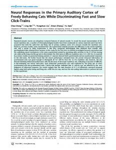
FIG. 4. Phoneme classification based on the population response. Classification masks for three unvoiced plosives 共/p/, /t/, /k/兲 and three unvoiced fricatives 共/f/, /s/, /b/兲 sorted by neurons’ best frequency 共A兲, best scale 共B兲 and best rate 共C兲. Gray scale indicates the importance of the presence 共black regions兲 or absence 共white regions兲 of neural response for the classification of that phoneme. The output of each phoneme classifier is a scalar, computed as the sum of the population PSTH multiplied by the mask. Thus the order of the mask/PSTH is irrelevant to the output of the classifier.

nemes, given the natural acoustic variability among samples of the same phoneme during continuous speech. To delineate perceptual boundaries implied by the responses to the phonemes, we trained a linear classifier for each phoneme to separate it from all others, based on the PSTHs of the neural population.36 To determine the identity of a novel phoneme, the population response was applied to all the classifiers, each computing the likelihood of its designated phoneme. The classifier indicating the maximum likelihood was taken as the identity of the input phoneme. To train and test the classifiers, we divided the speech data into 100 train and test subsets. In each subset, 90% of the data was randomly chosen for training and the remaining 10% was used for testing. The classification accuracy and the confusion matrices reported here are the average results from these 100 subsets. Once trained, each linear classifier can be viewed as a mask that selects, by multiplication with the population response, the neurons and response latencies that most effectively distinguish the associated phoneme from all others. Figure 4 displays the masks computed for the unvoiced consonants /p/, /t/, /k/, /f/, /s/, /b/. The masks are ordered in the same way as the PSTHs in Fig. 3共A兲 共i.e., by BF, best scale, and best rate兲. In the masks, black regions signify neurons and response latencies for which a strong response provides evidence for presence of the phoneme, and white regions signify strong responses that provide evidence against that phoneme. The masks in Fig. 4 differ from the mean neural responses in Fig. 3共A兲 in that they emphasize the unique features of each phoneme. For example, the mean responses 906

J. Acoust. Soc. Am., Vol. 123, No. 2, February 2008

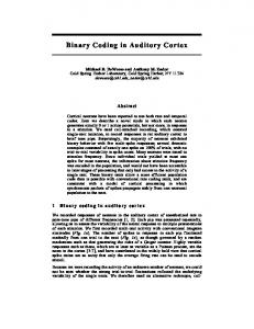
FIG. 5. Neural and human phoneme confusions, and phonemes acoustic similarity. Consonant confusion matrices from neural phoneme classifiers 共left panels兲 and human psychoacoustic studies 共Ref. 17兲 共middle panels兲. Gray scale indicates the probability of reporting a particular phoneme 共column兲 for an input phoneme 共row兲. 共Right panels兲 The acoustic similarity between phoneme pairs defined as the Euclidian distance between their average auditory spectrograms. 共A兲 Confusion matrices and phonemic distances for unvoiced consonants. Dashed lines separate the plosives /p/, /t/, /k/ from fricatives /f/, /s/, /b/. 共B兲 Confusion matrices and phonemic distances for voiced consonants. Dashed lines separate the plosives /b/, /d/, /+/ from fricatives /v/, /ð/, /z/ and the nasal consonants /m/ and /n/ from the rest.

to /b/ 共Fig. 3共A兲-II兲 indicate strong responses in high and medium BF neurons, but in the masks the mid-BF neurons 共2 kHz兲 are given higher weights. This differential weighting reflects the fact that both /b/ and /s/ evoke strong responses from high BF neurons, but only /b/ evokes responses from the mid-BF neurons. Similarly, the /p/, /t/, /k/ masks reflect only the features that distinguish these phonemes from each other. The BF masks 共Fig. 4共A兲兲 emphasize the low 共750 Hz兲, high 共⬎2 kHz兲, and medium 共0.3– 1.5 kHz兲 spectral regions for the /p/, /t/, /k/ bursts, respectively. Note also how the rate masks 共Fig. 4共C兲兲 distinguish plosives /p/, /t/, /k/ from the long fricatives /s/, /b/ by enhancing the regions outlined in the rectangle, namely the slow rates of the fricatives 共⬍11 Hz兲 relative to the faster rates of the plosives. It should be noted that the classifier performance does not depend in any way on the order of the neural responses, which is solely used for analysis and display purposes. The extent to which the neural phoneme representations can account for the perception of individual phoneme exemplars can be assessed by studying the pattern of pair-wise confusions by the classifier. Figure 5共A兲 shows the confusion matrix measured from classifications of the neural data. Labels along each row indicate the phoneme presented, and columns report the probability of the phoneme output by the classifier.17,37 The classifier was trained on two sets of data. In a small set of 20 neurons, we succeeded in measuring responses to 330 s of speech 共90 sentences兲 to be used in the training; these are shown in Fig. 5. In a larger set, training was based on responses from all sampled neurons in which at least 90 s of speech stimuli 共30 sentences兲 were presented; these results are shown in Fig. 7 of the Appendix. In an ideal case in which all phonemes were accurately identifiable, we would expect to see a diagonal confusion matrix. Offdiagonal values represent misidentification. The phonemes Mesgarani et al.: Classification of phonemes in auditory cortex

are arranged based on voiced-unvoiced and plosive, fricative, nasal consonant categories to facilitate comparison with a previous study of human perception17,37 共replicated in Fig. 5共B兲兲. The dashed boxes delineate the three major phoneme categories: plosives, fricatives, and nasals. In both neural and perceptual data, phonemes within each category—plosives 共/p/, /t/, /k/兲, fricatives 共/f/, /s/, /b/兲, and nasals 共/m/, /n/兲—tend to be more confusable within the group than across categories. The correlation coefficient between the complete neural and perceptual matrices is 0.78 共p = 0.0002, randomized t test兲. Ignoring the confusions between voiced and unvoiced consonants improves the similarity to 0.86, with a correlation of 0.95 for only the unvoiced consonants and 0.71 for their voiced counterparts. At least some of the difference between confusion matrices reflects noise due to limited sampling of neural responses, and/or limited data for training the phoneme classifiers. For example, when we computed the same confusion matrix for the entire population of 90 neurons 共trained only on 90 s of speech兲, the correlation between neural and human confusion matrices fell to 0.70 共p = 0.001兲, a change that may reflect the added dimensions and free parameters as new neurons are included in the analysis, while the amount of training data decreases at the same time. 共Appendix; Fig. 7兲. Alternatively, we explored the sensitivity of the classification in Fig. 5 to the number of neurons included 共using the same training material兲. As expected, the results indicate that percentage of correct classification 共averaged across all consonant phonemes兲 improves as the number of randomly selected neurons is increased 共Appendix; Fig. 8兲. More detailed exploration of this issue should take into account the differential contribution of specific neurons to different phonemes, e.g., high BF neurons to the classification of /s/ and /b/. Finally, we also explored the extent to which both the neural and human confusion matrices are a reflection of the acoustic similarity 共or “distances”兲 among the phonemes at the level of the auditory spectrograms 共see Sec. II兲. Figure 5 illustrates that such a phoneme “similarity matrix” fundamentally resembles the human and neural confusion matrices 共with correlation coefficients of 0.66 and 0.93, respectively兲. In fact, the neural matrix encodes remarkably well the details of the phoneme acoustic similarity, such as the confusions between /v/ and the nasals /m/, /n/, and also between /ð/ and the voiced consonants /b/, /d/, /+/. IV. DISCUSSION

Neuronal responses to continuous speech in the primary auditory cortex of the naive ferret reveal an explicit multidimensional representation that is sufficiently rich to support the discrimination of many American English phonemes. This representation is made possible by the wide range of spectro-temporal tuning in A1 to stimulus frequency, scale and rate. The great advantage of such diversity is that there is always a unique subpopulation of neurons that responds well to the distinctive acoustic features of a given phoneme and hence encodes that phoneme in a high-dimensional space. As an example, consider the perception of the plosive consonant /k/ in a CV syllable, which is identified by a conJ. Acoust. Soc. Am., Vol. 123, No. 2, February 2008

junction of several acoustic features: an initial silent voiceonset time 共VOT兲, an onset burst of spectrally broad noise, and the direction of the following formant transitions.23 Each of these features can be encoded in the cortical responses along different dimensions. Thus, neurons selective for broad spectra respond selectively to the noise burst. Rapid neurons respond well following the VOT, whereas directional neurons selectively encode the vowel formant transitions. In this manner, /k/ is encoded robustly by a rich pattern of activation that varies in time across the neural population. This neuronal activation pattern constitutes the phoneme representation in A1 and presumably forms the input to a set of neural “phoneme classifiers” in higher auditory areas. If one acoustic feature is distorted or absent, the pattern along the other dimensions 共and hence the percept兲 remains stable. We have focused here on describing a few prominent features of the response distributions that correspond to wellknown distinctive acoustic features of the consonants considered.24 There are clearly many other aspects and more details of the responses that reflect intricate articulatory gestures, contextual effects, or speaker-dependent variability that can only be reliably considered with a much larger sample of responses. One example is the distribution of the directionality index of the responses in the neighborhood of a consonant,38 an attribute that would indicate whether the formants are upward or downward sweeping, or if they are converging towards or diverging away from a locus frequency. Humans confuse the phonemes of their native tongue when placed in unusual or noisy contexts. Typically, phonemes that share some acoustic features tend to be more confusable than those that do not. This was confirmed by the similarity we found between the acoustic distance and the human confusion matrices. Similarly, since A1 responses in our naive ferrets also preserve the relative acoustic distances between the phonemes 共as they would presumably for other complex sounds兲, we are led to the conjecture that human phoneme perception can 共in principle兲 be explained in large measure by basic auditory representations such as the auditory spectrogram and the cortical spectro-temporal analysis common to many mammalian 共and also avian兲 species.6,9,10,39,40 The representation of phonemic features across a population of filters tuned to BF, scale and rate suggests a strategy for improved speech recognition systems, and further study may reveal additional strategies for speech processing. However, many questions about the neural representation of phonemes still remain unanswered; for example, how can one extrapolate from such neurophysiological findings to the human perceptual ability to perceive phonemes categorically 共also found in monkeys,11 cats,8 chinchillas,3 birds9 and rats,41兲, and to shift categorical boundaries arbitrarily between phoneme pairs? While the human ability to discriminate native phonemes is the result of many years of training, naïve ferrets lack such a history. Hence ferret perception of clean phonemes may be comparable to humans perception of noisy phonemes. In both cases, confusion patterns would reflect the acoustic distances between the phonemes. However, if ferrets were trained to actively discriminate phonemes, it is Mesgarani et al.: Classification of phonemes in auditory cortex

907

FIG. 6. Joint distribution of neural parameters. Joint distributions of best frequency, best rate 共A兲, best frequency, best scale 共B兲 and best rate, best scale 共C兲 of 90 neurons.

likely that dimensions useful for this specific discrimination would be emphasized, creating the heightened sensitivity necessary to perform the task. This is presumably what happens in humans as they learn the phonemes of a given language, and what the classifier essentially simulates in our analysis when it learns the masks and boundaries that enable robust phoneme discriminations. Therefore, from a neural perspective, one may view the masks as either a subsequent layer of synaptic weights or as pattern of behaviorally driven plasticity of A1 receptive fields—the end result of perceptual learning in which neurons adapt their tuning along the dimensions appropriate for the phoneme discrimination task. This same general principle would apply to the discrimination between members of any set of complex sound, using frequency, rate and scale as well as additional cortical response dimensions, such as pitch, spatial location, and loudness. ACKNOWLEDGMENTS

This work was supported by the National Institutes of Health 共Grant Nos. R01DC005779 and F32DC008453兲, the

FIG. 8. Dependence of phoneme classification accuracy to the number of neurons. Classification accuracy as a function of the number of neurons used by the classifier. The dashed line indicates chance performance 共7% for 14 phonemes兲 共see Sec. II for details兲.

Air Force Office of Scientific Research and the Southwest Research Institute. APPENDIX

Here we provide additional information regarding: 共A兲 uniformity of the sampling of the neural parameters; 共B兲 the phoneme confusions from an SVM recognizer using a larger number of neurons, but with significantly fewer speech responses on which to train the classifier; 共C兲 an exploration of the recognition accuracy with fewer numbers of neurons. 1. Joint distribution of neural parameters

To ensure that the response patterns in Figs. 2共A兲 and 3共A兲 are representative of the neural population in the cortex, we examined the uniformity of the coverage of the parameters of neural STRFs in our sample of 90 neurons. Specifically, the joint distributions of the different neural receptive field parameters 共best frequency, best scale, and best rate兲 are shown in the three panels of Fig. 6, revealing fairly uniform coverage over all frequencies, bandwidths, and different dynamics 共see Sec. II for further details兲. 2. Phoneme confusions from 90 neurons

Phoneme confusions derived from responses of the entire population of 90 neurons, but using only 90 s of speech, are displayed in Fig. 7. The correlation coefficient between the neural and human phoneme confusion 共0.70; p = 0.001兲 is still reasonable but is significantly less than that of the patterns in Fig. 8 共see method for more details兲. 3. Dependence of phoneme classification accuracy to the number of neurons FIG. 7. Phoneme confusions from 90 neurons. 共Left column兲 Consonant confusion matrices from neural phoneme classifiers using entire population of 90 neurons and 90 s of speech. 共Right column兲 human psychoacoustic studies. Gray scale indicates the probability of reporting a particular phoneme 共column兲 for an input phoneme 共row兲. 共a兲 Confusion matrices for unvoiced consonants. Dashed lines separate the plosives /p/, /t/, /k/ from fricatives /f/, /s/, /b/. 共b兲 Confusion matrices for voiced consonants. Dashed lines separate the plosives /b/, /d/, /g/ from fricatives /v/, /ð/, /z/ and the nasal consonants /m/ and /n/ from the rest. 908

J. Acoust. Soc. Am., Vol. 123, No. 2, February 2008

The number of neurons is a crucial variable in determining the accuracy of the phoneme classification as illustrated in the results of Fig. 8. Here the classification accuracy was computed as a function of the number of neurons used in training the classifier. For each condition, 100 random subsets of neurons were taken and the classification accuracy was averaged over all subsets. Note that the accuracy based Mesgarani et al.: Classification of phonemes in auditory cortex

on the 20 neurons in this plot is still only at 37% 共7% is chance performance兲. Presumably, adding more neurons increases the performance. 1

R. P. Lippmann, “Speech recognition by machines and humans,” Speech Commun. 22, 1–15 共1997兲. 2 S. Greenberg, W. Ainsworth, A. N. Popper, and R. R. Fay, Speech Processing in the Auditory System 共Springer-Verlag, New York, 2004兲, Vol. 18. 3 P. K. Kuhl and J. D. Miller, “Speech perception by the chinchilla: Voicedvoiceless distinction in alveolar plosive consonants,” Science 190, 69–72 共1975兲. 4 P. K. Kuhl and D. M. Padden, “Enhanced discriminability at the phonetic boundaries for the place feature in macaques,” J. Acoust. Soc. Am. 73共3兲, 1003–1010 共1983兲. 5 P. K. Kuhl and D. M. Padden, “Enhanced discriminability at the phonetic boundaries for the place feature in macaques,” J. Acoust. Soc. Am. 73共3兲, 1003–1010 共1983兲. 6 K. R. Kluender, A. J. Lotto, L. L. Holt, and S. L. Bloedel, “Role of experience for language-specific functional mappings of vowel sounds,” J. Acoust. Soc. Am. 104共6兲, 3568–3582 共1998兲. 7 F. Pons, “The effects of distributional learning on rats’ sensitivity to phonetic information,” J. Exp. Psychol. Anim. Behav. Process 32共1兲, 97–101 共2006兲. 8 R. D. Hienz, C. M. Aleszczyk, and B. J. May, “Vowel discrimination in cats: Acquisition, effects of stimulus level, and performance in noise,” J. Acoust. Soc. Am. 99共6兲, 3656–3668 共1996兲. 9 M. L. Dent, E. F. Brittan-Powell, R. J. Dooling, and A. Pierce, “Perception of synthetic /ba/-/wa/ speech continuum by budgerigars 共Melopsittacus undulatus兲,” J. Acoust. Soc. Am. 102共3兲, 1891–1897 共1997兲. 10 A. J. Lotto, K. R. Kluender, and L. L. Holt, “Perceptual compensation for coarticulation by Japanese quail 共Coturnix coturnix japonica兲,” J. Acoust. Soc. Am. 102共2 Pt 1兲, 1134–1140 共1997兲. 11 M. Steinschneider, Y. I. Fishman, and J. C. Arezzo, “Representation of the voice onset time 共VOT兲 speech parameter in population responses within primary auditory cortex of the awake monkey,” J. Acoust. Soc. Am. 114共1兲, 307–321 共2003兲. 12 M. Steinschneider, D. Reser, C. E. Schroeder, and J. C. Arezzo, “Tonotopic organization of responses reflecting stop consonant place of articulation in primary cortex 共A1兲 of the monkey,” Brain Res. 674, 147–152 共1995兲. 13 M. Steinschneider, I. O. Volkov, Y. I. Fishman, H. Oya, J. C. Arezzo, and M. A. Howard, “Intracortical responses in human and monkey auditory cortex support a temporal processing mechanism for encoding of the voice onset time phonetic parameter,” Cereb. Cortex 15, 170–186 共2005兲. 14 J. J. Eggermont and C. W. Ponton, “The neurophysiology of auditory perception: From single units to evoked potentials,” Audiol. Neuro-Otol. 7共2兲, 71–99 共2002兲. 15 C. P. Hung, G. K. Kreiman, T. Poggio, and J. J. DiCarlo, “Fast readout of object identity from macaque inferior temporal cortex,” Science 310, 863– 866 共2005兲. 16 K. Walker, B. Ahmed, and J. W. Schnupp, “Linking cortical spike pattern codes to auditory perception,” J. Cogn Neurosci., Oct 5 共Epub兲 共2007兲. 17 G. Miller and P. Nicely, “An analysis of perceptual confusions among some English consonants,” J. Acoust. Soc. Am. 27, 338–352 共1955兲. 18 F. E. Theunissen, S. V. David, N. C. Singh, A. Hsu, W. E. Vinje, and J. L. Gallant, “Estimating spatio-temporal receptive fields of auditory and visual neurons from their responses to natural stimuli,” Network 12共3兲, 289– 316 共2001兲. 19 D. J. Klein, J. Z. Simon, D. A. Depireux, and S. A. Shamma, “Stimulus-

J. Acoust. Soc. Am., Vol. 123, No. 2, February 2008

invariant processing and spectrotemporal reverse correlation in primary auditory cortex,” J. Comput. Neurosci. 20共2兲, 111–136 共2006兲. 20 S. Seneft and V. Zue, “Transcription and alignment of the timit database,” J. S. Garofolo, editor, National Institute of Standards and Technology 共NIST兲, Gaithersburg, MD 共1988兲. 21 X. Yang, K. Wang, and S. A. Shamma, “Auditory representation of acoustic signals,” IEEE Trans. Inf. Theory 38共2兲, 824–839 共Special issue on wavelet transforms and multi-resolution signal analysis兲 共1992兲. 22 S. V. David and J. L. Gallant, “Predicting neuronal responses during natural vision,” Network 16共2–3兲, 239–260 共2005兲. 23 P. Ladefoged, A Course in Phonetics, 5th ed. 共Harcourt Brace, Orlando, 2006兲. 24 K. N. Stevens, Acoustic Phonetics 共MIT Press, Cambridge, MA, 1980兲. 25 S. Shamma, “Speech processing in the auditory system. Part I: The representation of speech sounds in the responses of the auditory-nerve,” J. Acoust. Soc. Am. 78共5兲, 1612–1621 共1985兲. 26 E. D. Young and M. B. Sachs, “Representation of steady-state vowels in the temporal aspects of the discharge patterns of populations of auditory nerve fibers,” J. Acoust. Soc. Am. 66, 1381–1403 共1979兲. 27 C. E. Schreiner, H. L. Read, and M. L. Sutter, “Modular organization of frequency integration in primary auditory cortex,” Annu. Rev. Neurosci. 23, 501–529 共2000兲. 28 H. L. Read, J. A. Winer, and C. E. Schreiner, “Functional architecture of auditory cortex,” Curr. Opin. Neurobiol. 12共4兲, 433–440 共2002兲. 29 D. A. Depireux, J. Z. Simon, D. J. Klein, and S. A. Shamma, “Spectrotemporal response field characterization with dynamic ripples in ferret primary auditory cortex,” J. Neurophysiol. 85, 1220–1234 共2001兲. 30 L. A. Chistovich and V. V. Lublinskaya, “The center of gravity effect in vowel spectra and critical distance between the formants: Psychoacoustical study of the perception of vowel-like stimuli,” Hear. Res. 1, 185–195 共1979兲. 31 We emphasize that this response pattern is unlikely to be due to a nonuniform sampling of the scale and frequency variables, since no such bias in the joint distribution of the scale frequency is evident in Fig. 6共A兲. Furthermore, note that high scale neurons can be driven well by spectra with low frequencies as in phoneme /o/. The opposite is true for vowel /e/ where low scale units are driven well by high frequency energy. 32 W. Klein, R. Plomp, and L. C. Pols, “Vowel spectra, vowel spaces and vowel identification,” J. Acoust. Soc. Am. 48共4兲, 999–1009 共1970兲. 33 T. F. Quatieri, Discrete-Time Speech Signal Processing: Principles and Practice 共Prentice–Hall, Englewood Cliffs, NJ, 2002兲. 34 O. Deshmukh, C. Espy-Wilson, A. Salomon, and J. Singh, “Use of temporal information: Detection of the periodicity and aperiodicity profile of speech,” IEEE Trans. Speech Audio Process. 13共5兲, 776–786 共2005兲. 35 D. Bendor and X. Wang, “The neuronal representation of pitch in primate auditory cortex,” Nature 共London兲 436, 1161–1165 共2005兲. 36 V. N. Vapnik, The Nature of Statistical Learning Theory 共Springer, New York, 1995兲. 37 J. B. Allen, Articulation and Intelligibility 共Morgan and Claypool, 2005兲. 38 D. Depireux, J. Z. Simon, and S. Shamma, “Measuring the dynamics of neural responses in primary auditory cortex,” Comments in Theoretical Biology 5共2兲, 89–118 共1998兲. 39 N. Kowalski, D. Depireux, and S. Shamma, “Analysis of dynamic spectra in ferret primary auditory cortex: Prediction of single-unit responses to arbitrary dynamic spectra,” J. Neurophysiol. 76共5兲, 3524–3534 共1996兲. 40 L. M. Miller, M. A. Escabi, H. L. Read, and C. E. Schreiner, “Spectrotemporal receptive fields in the lemniscal auditory thalamus and cortex,” J. Neurophysiol. 87, 516–527 共2002兲. 41 C. T. Novitski et al., Program 800.18/Poster E45, Neural coding of speech sounds in naïve and trained rat primary auditory cortex, Society for Neuroscience, Atlanta 共2006兲.

Mesgarani et al.: Classification of phonemes in auditory cortex

909