Practical Routing in Delay-Tolerant Networks Evan P. C. Jones
[email protected]
Lily Li
[email protected]
Paul A. S. Ward
[email protected]
Electrical & Computer Engineering University of Waterloo Waterloo, Ontario, Canada
ABSTRACT
Keywords
Delay-tolerant networks (DTNs) have the potential to connect devices and areas of the world that are under-served by current networks. A critical challenge for DTNs is determining routes through the network without ever having an end-to-end connection, or even knowing which “routers” will be connected at any given time. Prior approaches have focused either on epidemic message replication or on knowledge of the connectivity schedule. The epidemic approach of replicating messages to all nodes is expensive and does not appear to scale well with increasing load. It can, however, operate without any prior network configuration. The alternatives, by requiring a priori connectivity knowledge, appear infeasible for a self-configuring network. In this paper we present a practical routing protocol that only uses observed information about the network. We designed a metric that estimates how long a message will have to wait before it can be transferred to the next hop. The topology is distributed using a link-state routing protocol, where the link-state packets are “flooded” using epidemic routing. The routing is recomputed when connections are established. Messages are exchanged if the topology suggests that a connected node is “closer” than the current node. We demonstrate through simulation that our protocol provides performance similar to that of schemes that have global knowledge of the network topology, yet without requiring that knowledge. Further, it requires a significantly smaller quantity of buffer, suggesting that our approach will scale with the number of messages in the network, where replication approaches may not.
Delay tolerant network, Route metrics, Routing
Categories and Subject Descriptors C.2.2 [Network Protocols]: Routing protocols
General Terms Design, Performance
Permission to make digital or hard copies of all or part of this work for personal or classroom use is granted without fee provided that copies are not made or distributed for profit or commercial advantage and that copies bear this notice and the full citation on the first page. To copy otherwise, to republish, to post on servers or to redistribute to lists, requires prior specific permission and/or a fee. SIGCOMM’05 Workshops, August 22–26, 2005, Philadelphia, PA, USA. Copyright 2005 ACM 1-59593-026-4/05/0008 ...$5.00.
1. Introduction Delay-tolerant networks (DTNs) have the potential to connect devices and areas of the world that are not well-served by current networking technology. Instead of relying on end-to-end network connectivity, DTNs take advantage of temporary connections to relay data in a fashion similar to the postal network [6]. These networks could be useful in scenarios ranging from interconnecting sensors to connecting remote regions of the world. One obstacle that currently limits deployment of these networks is that it is difficult to determine how to get data from the source to the destination. Current DTN-like networks have been built using static routing [11, 14]. This is an effective approach for small networks with simple topologies. However, the benefit of these networks will increase if they can be scaled to service larger areas. To achieve this goal, routing protocols are needed to automate network configuration. This paper presents a routing protocol designed to be easy to deploy in order to accelerate the use of DTNs. This philosophy led to three design goals. First, the routing must be self-configuring. This is critical for equipment that may be deployed far from network experts, and to maintain connectivity in the face of failure. Second, the protocol must provide acceptable performance over a wide variety of connectivity patterns. Finally, it must make efficient use of buffer and network resources, being scalable with the number of messages delivered. We use a simplified version of the DTN model presented by Jain et al. [9]. We model the network as an undirected graph where nodes are connected by bidirectional links called contacts. A contact represents an opportunity for the connected nodes to exchange data. It begins at some point in time and persists for a finite duration. When a contact is up (i.e. the nodes that form the contact are connected), it has a constant link bandwidth and negligible delay. Bidirectionality implies that our protocol will not operate in networks with unidirectional links, such as satellite connections. The assumption of constant link bandwidth and delay means that routing performance may be degraded if these parameters vary. The remainder of this paper is organized as follows. First, we discuss the previous work on the delay-tolerant routing problem, demonstrating its limitations. In Section 3, we justify our design decisions, and detail our overall protocol. We compare the performance of our protocol with previous work in Section 4. Finally, we discuss our conclusions and future work.
2.
Related Work
Our protocol is a shortest path routing protocol for delay-tolerant networks. Its design is based on routing in traditional networks, but some design decisions were modified for this new environment. First we discuss some of the issues in selecting a path metric and present the metric we use. Next we investigate when to make routing decisions, and finally how to distribute topology information.
resolve this problem, we follow the same approach as Jain et al. and choose to minimize the end-to-end delay [9]. This reduces the amount of time a message occupies buffers in the network, which intuitively should reduce the number of messages dropped, assuming that buffer overflow is the primary cause of loss. In a delay-tolerant network, the end-to-end delay has four components. First, the message must wait for the next contact to arrive (waiting time). Next, the data queued ahead of the current message must be delivered (queuing delay). The message must then be transmitted (transmission delay), and finally the signal must propagate to the next hop (latency). Delay is an attractive metric because these four factors can be combined into a single number, assuming that sufficient information is available. However, to simplify the discussion in this paper, we assume that links have a very high throughput and low latency, which means that the waiting time is the only significant factor. To account for links that have significant latency, these factors must be added to the expected waiting time to compute the final metric. A variety of metrics for minimizing the end-to-end delay in a DTN have been explored by Jain et al. [9]. However, most of them require knowledge of future contact arrival times. An exception is the minimum expected delay (MED). This metric assigns a cost to each edge equal to the expected waiting time plus the transmission delay. Once this value is computed, the contact schedule is not needed. Assuming that message arrival times are uniformly distributed, the waiting time probability distribution is a piecewise linear function. It is a straightforward application of basic probability to compute the expected value. We propose a variant of MED we call the minimum estimated expected delay (MEED). Instead of computing the expected waiting time using the future contact schedule, MEED uses the observed contact history. Previous work has shown that mobility observations can make predictions with accuracy greater than 80% [17]. This metric differs from previous work because it tries to make a reasonable prediction about aggregate mobility over the period of time it takes to deliver a message through the DTN, which could be hours or days. By contrast, mobility prediction for cellular systems attempts to guess the next cell location of a mobile node, which requires predicting mobility for the next few minutes. To compute this metric, a node records the connection and disconnection times of each contact over a sliding history window. The sliding window size is a tuning parameter that can be adjusted independently at each node. If the window size is very large, then the metric will change very slowly. This is good to avoid perturbations caused by random changes in the contact schedule, but also means that it reacts slowly to permanent changes in the topology. Conversely, a small window reacts quickly to changes, which means the metric will be more sensitive to random fluctuations. When the local link state table changes, the update must be propagated to all nodes in the network. This is an expensive operation. To reduce the overhead, a node may optionally suppress updates that it decides are unnecessary. However, it is essential that it continues to make routing decisions using the table that it last advertised. Our simple implementation propagates an update only if at least one link weight changed by more than 5%, or if a new contact has been added.
3.1.
3.2.
Work on routing protocols for multi-hop wireless networks shows that it is possible to automatically route in networks, even when nodes are mobile and the link quality varies. There is a huge body of work on routing protocols [12, 13, 1, 15] and metrics [16, 4, 5] for this environment. However, these protocols and metrics find end-to-end paths, and do not support communication between nodes in different network partitions. One of the earliest proposals for routing in disconnected networks is epidemic routing [19]. It relies on replicating messages through random exchanges between nodes until all nodes have a copy of every message. Each node has a buffer where it stores these messages. When it comes into contact with another node, the two nodes exchange messages until their buffer contents are synchronized. This approach can achieve high delivery ratios, and operates without knowledge of the communication pattern. It is well-suited to networks where the contacts between nodes are unpredictable. Unfortunately, it is very expensive in terms of the number of transmissions and buffer space. In particular, it does not appear that this approach can scale as the number of messages in the network grows. The critical resource in epidemic routing is the buffer. An intelligent buffer management scheme can improve the delivery ratio over the simple FIFO scheme [3]. The best buffer policy evaluated is to drop packets that are the least likely to be delivered based on previous history. If node A has met B frequently, and B has met C frequently, then A is likely to deliver messages to C through B. Similar metrics are used in a number of epidemic protocol variants [3, 10, 18]. This approach takes advantage of physical locality and the fact that movement is not completely random. However, these protocols still transmit many copies of each message, making them very expensive. An approach that uses a single copy of each message is presented by Jain et al. [9]. They assume that the contact schedule is completely known in advance, and use this knowledge to create a number of routing metrics. Their results show that the efficiency and performance increases with the amount of information used for the metric. The weakness of this approach is that each node must have access to accurate schedule data. To provide this information, the routing must be manually configured with the contact schedules, which must be repeated each time the schedule changes. Handorean et al. explore alternatives for distributing connectivity information, but they still assume that each node knows its own connectivity perfectly [7]. It is unclear how the performance will be affected if the schedules are imprecise, which is the typical case in the real world, or if there are failures which alter the communication pattern.
3.
Routing Design
Path Metrics For DTNs
Paths must be carefully selected to extract the best performance from a network. In a DTN, the primary requirement is that messages are reliably delivered. Thus, delivery ratio is a very important metric. Unfortunately, it is not clear how a metric can be constructed to directly maximize delivery ratio along a path. To
Routing Decision Time
The earliest opportunity that the path for a message can be decided is at the source, which is called source routing. This is a simple approach but it is inappropriate for delay-tolerant networks because as the message travels closer to the destination, the nodes will likely have more recent and accurate information about the
D
A
D
2
2
2
6
2 B
B
C
3
8
B
4
1
C
C
3
Figure 2: Routing loop caused by short circuit routing
0
A
A
(a)
(b)
Figure 1: Per-contact routing
destination’s connectivity. hence it seems natural that these intermediate nodes can make better decisions than the source. The next time to make forwarding decisions is when a message arrives at each intermediate node, which is called per-hop routing. When the message arrives, the node determines the next hop for the destination and places it in a queue for that contact. This is also not a good solution for DTNs, as changes to the topology could occur after the message arrives. This would result in the message waiting to be forwarded over a sub-optimal link. In order to make routing decisions with the best possible information, we use what we call per-contact routing. Instead of computing the next hop for a message in advance, the routing table is recomputed each time a contact arrives. This assures that each routing decision is made with the most recent information. The disadvantage is that this approach uses more processing resources, as the routing is recomputed frequently. Additionally, the routing must be recomputed before any messages may be forwarded. Thus, there may be some additional delay before a link will be used. As long as the processing power of the nodes is appropriate for the size of the network, this delay will not be significant. However, it may be a limiting factor in scaling this approach to very large networks. Contacts that arrive infrequently have a high minimum expected delay because the waiting time is very long. Thus, the shortest paths will not use these links. However, these links might be very good when they are available. Since we recompute the routing table when a contact arrives, we can take advantage of these links by temporarily assigning a cost of zero to any contact that is available. This ”short circuits” the routing decisions made by the linkstate protocol, allowing messages to take advantage of good timing. This is similar to the approach used in some epidemic routing variants [3, 18], and to what Handorean et al. call a ”path update” [7]. Per-contact routing combined with this temporary short circuiting is effective for delay-tolerant networks because it guarantees that decisions are always made with the most recent information possible, and it can take advantage of serendipitous contact arrivals to make the routing more efficient. For example, imagine we have a network with four nodes. Node A has a message for node D. There are two possible next hops: B with a total path cost of 5, and C with a total path cost of 10. This topology is shown in Figure 1(a). Thus, the current routing state says the message should wait for B to reach D. However, node C connects first. Thus, the cost to go from A to C becomes zero, as shown in Figure 1(b). With per-hop or source routing, the message would remain queued at A waiting for the path with cost 5, through node B. However, per-contact routing takes advantage of this unforeseen contact and delivers the message to C, where it will wait for a path with cost 2.
3.3.
Impact of Deferring Routing Decisions
Making routing decisions as late as possible seems like a clear win for delay-tolerant networks because it allows the path taken by a message to change while it is in transit. For example, consider the situation where the next hop for a message never arrives due to a failure. Eventually the routing system can give up waiting for the contact to arrive. At this point, source or per-hop routing would drop the message because the connection it was waiting to use has gone down. However, per-contact routing will simply wait for an alternate contact. Unfortunately, this choice does have one drawback. Link state routing is loop free only if the same topology is used to make all the routing decisions along the path of a message. Source routing guarantees that this occurs because all the routing decisions are made at the source. In connected networks, per-hop routing assumes that the topology does not change while the message is in transit. This is reasonable since the end-to-end delay is measured in milliseconds, and topology changes are relatively rare, but this assumption does not hold for DTNs. If the link weights change while the data is in transit, it is possible for a packet to get passed between two nodes indefinitely. For a loop to occur, the link weights must change enough so that when the packet gets to one of the nodes, the routing directs the packet back the way it came. A situation where this loop could occur in a DTN is shown in Figure 2. Initially, node B has a message for node A, and the shortest path is BCA. When node C connects to B, the message is forwarded to C. Now, imagine that the cost of the contact BA decreases because A connects to B. Meanwhile, the cost of the CA contact increases to 6 because C has not been connected to A for some time. At this point, the situation is the mirror image of how it began. The message would have been delivered if it had stayed at B. Now if B connects to C, the message will be sent back to B. If the connectivity pattern is periodic, the message will bounce between B and C indefinitely. Short circuit routing aggravates this problem because the link cost between B and C no longer matters, so the link costs need to fluctuate less. This problem could be mitigated by adding some hysteresis. In order to backtrack, the path must improve upon the next best path by some threshold. The threshold could increase if a node is revisited multiple times. We do not implement this solution in our simulations because it would add a significant amount of complexity. However, a real implementation would need a solution because while this situation seems unlikely to occur, it would cause significant disruption. 3.4.
Topology Distribution
Once we have costs for individual links, the information needs to be distributed throughout the network. Traditional networks typically use link-state or distance vector algorithms for this purpose, although other choices are possible. We chose to implement a linkstate routing algorithm for two reasons. The primary reason is that there is a natural match between flooding in link-state algorithms and epidemic message distribution. Flooding distributes a copy of each link state table to all nodes. Epidemic replication distributes
Disconnected connect
Topology Summary Wait Send Topology Summary connection idle Wait for Topology Summary received topology summary
Exchange Updates Wait to Send Updates connection idle
topology changed
Wait for Updates updates received
Forwarding Send Messages connection idle
Figure 3: The epidemic link state protocol state machine a copy of each message to all nodes. Thus, we can implement a link-state protocol in a DTN using an epidemic algorithm, which has been shown to be very robust. The secondary reason we chose to implement link-state routing is that it provides the complete topology at each node, which allows the topology to be updated in a single contact. Thus, if a node has been disconnected for a long time it can obtain the entire topology in a single exchange with any other node. A distance vector algorithm would only distribute paths that pass through the other node. Link-state routing does have its disadvantages. First, each node must store the entire topology in its routing tables, which could be larger than the state required for distance vector routing. Second, merging topology information from multiple nodes becomes more complicated because there is more information to be synchronized. 3.5.
An Epidemic Link State Protocol
Upon connection, nodes exchange summary vectors that list all the link state tables the nodes have received. Each table is tagged with a sequence number which permits the nodes to determine which ones are the most recent. The nodes exchange any missing updates so that they both have the same topology state. Then they recompute their routing tables and finally, messages that should be routed through the other node are forwarded. Since we use percontact routing, the metric for each link is temporarily set to zero to represent the fact that messages can be immediately sent to the other node. The protocol state, shown in Figure 3, is maintained individually for each connection. To estimate the overhead of this protocol the size of each protocol message must be determined. There are two protocol messages exchanged: summary vectors and topology updates. The summary vector contains one (source id, sequence number) pair for each node in the network. If we assume each value has a fixed length,
the size of this message scales linearly with the size of the network. The topology update contains a set of (source id, sequence number, link partner id, metric) tuples for each contact. In the worst case, the complete topology must be transmitted. In this case, the ), where is the number topology update has a size that is ( of nodes in the network, and is the degree of each node. If we assume that the average node degree is constant, this overhead also scales linearly with the size of the network. As a somewhat realistic example, if we encode these messages as arrays and assume each value is a 32-bit integer, an 802.11 packet containing 1 500 bytes of data can store an update with information about 92 links, which would be sufficient for a network with 15 nodes with an average degree of 6. Thus, the overhead is acceptable for small networks, but may be a problem for very large networks.
D
O ND
N
4. Performance Evaluation We evaluate the performance of five delay tolerant network routing protocols: the earliest delivery (ED) and minimum expected delay (MED) metrics [9], epidemic routing [19], a variant of MED that uses per-contact routing (MED Per Contact), and MEED. The ED protocol is used to illustrate the performance that can be achieved if complete and accurate contact schedule data is available. MED and MED Per-Contact are presented to investigate the performance of per-contact routing. Finally, MEED and Epidemic represent the performance of protocols that do not require schedule information. We used the DTN simulator written by Sushant Jain [9]. It is a simple discrete event simulator that uses FIFO, reliable links with fixed bandwidth and delay. 4.1.
Scenario
In order to give the scenarios a basis in reality, we used real mobility data from extensive wireless LAN traces from Dartmouth College [2]. These traces log the network activity of more than 2 000 users over two years. The trace files show when each user connects and disconnects to any of Dartmouth College’s 500 access points. This data is useful because while the mobility appears to be random, there are patterns that can be exploited [17]. We used the traces to create a scenario which represents users forming an adhoc DTN. In our scenario, mobile users carry computing devices with radios. When they are in range of another user, they exchange data. To transform the wireless LAN traces into an ad-hoc DTN, we consider two nodes to be connected when they are associated with the same access point at the same time. Access points are also DTN routers. In order to make the scenarios a manageable size, only a connected subset of the nodes from the wireless LAN trace are included. As an example, consider the wireless LAN scenario shown in Figure 4(a). At time 1, the trace file will show that the laptop user is connected to the access point on the left. Later, it moves out of range of the access point, and at time 2 it associates with the second access point. A DTN scenario that could be generated from this data is shown in Figure 4(b). One laptop and one access point from the original scenario were removed. 4.2.
Simulation Parameters
For each simulation we selected 30 nodes that have many opportunities to communicate over a period of one month. We include nodes that connect to another node at least ten times during the month. Each node selects another node at random, and bidirectional traffic is exchanged between the pair. Each node generates 6 messages every 12 hours during the month, but statistics are reported for only the messages generated during the second week.
Latency vs Buffer Space (30 nodes, 12 msgs/day/node, 10000 bytes/message) 100.0 90.0 80.0
2.
1.
70.0 Latency (hours)
2. 1. (a) Wireless LAN Scenario
(b) Ad-hoc DTN Scenario
60.0 50.0 40.0 30.0
Figure 4: Wireless trace converted into a DTN scenario
20.0 Delivery Ratio vs Buffer Space (30 nodes, 12 msgs/day/node, 10000 bytes/message)
ED MED MED Per Contact MEED Epidemic
10.0
1.000 0.0 0.0%
0.900
5.0%
10.0% Buffer Space (% Total Buffer)
15.0%
20.0%
0.800
Figure 6: Delivery latency with varying buffer size
Delivery Ratio
0.700 0.600 0.500
0.300
ED MED MED Per Contact MEED Epidemic
0.200 0.100 0.0
5.0
10.0 Buffer Space (% Total Traffic)
15.0
20.0
Figure 5: Delivery ratio with varying buffer size
Percent Improvement of Delivery Ratio
0.400
Improvement With Hop-By-Hop Flow Control (30 nodes, 12 msgs/day/node, 10000 bytes/message) 20.0% ED MED MED Per Contact 10.0% MEED 0.0% -10.0% -20.0% -30.0% -40.0% -50.0%
Each message is 10 000 bytes long. This workload represents two users exchanging small files or email messages. Each test is performed with 10 different network topologies. Our implementation does not support reactive fragmentation. We investigate how the performance of the protocols in the DTN scenario varies depending on the buffer size and the available bandwidth. In order to measure the effect of a single parameter, the default values for the buffer size and bandwidth are both very large. Two metrics are presented: delivery ratio and latency. We also evaluate the protocol overhead of MEED. 4.3.
Impact of Buffer Size
Looking at the graph of the delivery ratio over buffer size in Figure 5, we can immediately see that the buffer size has significant impact on the Epidemic protocol. As the buffer at each node becomes larger, the delivery ratio increases. Once the buffers are large enough to contain all the messages generated during the entire simulation (not shown due to space constraints), its delivery ratio matches ED. The Epidemic protocol only guarantees delivery if there is sufficient buffer to have a copy of every message at every node. If there is insufficient buffer, then some messages must be dropped. Thus, there is a very predictable relationship between the buffer size and the delivery ratio. The other protocols require much less buffer space because they use a single copy of each message. Only when the buffer size drops below 10% of the total traffic generated does the delivery ratio start to decrease. MEED’s delivery ratio is within approximately 5% of the best protocols. Considering that this protocol has no knowledge about the network topology, this is respectable. In a buffer constrained network, MEED has much better performance than Epidemic routing. Looking at the latency results, shown in Figure 6, we can see
-60.0% 0.0%
5.0%
10.0% Buffer Space (% Total Traffic)
15.0%
20.0%
Figure 7: Improvement with hop-by-hop flow control that the delay for the Epidemic protocol is much lower than the other protocols. This is because when the buffer is small, it drops the oldest messages which are then excluded from the delay computation. When the buffer is large enough, the delay for Epidemic matches ED. Using per-contact routing with MED decreases the latency significantly. MEED’s latency is similar to that of MED, even though it uses per-contact routing and uses a similar metric. The reason is that MEED must estimate the connectivity, so in some cases it makes bad routing decisions. These protocols use the “drop tail” queue policy. Thus, if there is insufficient buffer space when a message arrives, it is dropped. This source of loss could be reduced by using hop-by-hop flow control, so that the message is only sent to the next hop if sufficient buffer is available. This scheme has been shown to be effective at dealing with congestion in wireless sensor networks [8]. The improvement when using flow control is shown in Figure 7. This small change increases the delivery ratio when the buffer is the limiting factor. Without per-contact routing, flow control makes the delivery ratio decrease when the buffers are extremely small, because the congestion makes it impossible to deliver any messages in the network. Per-contact routing works around this problem by taking advantage of alternate routes. From these results, it seems that hopby-hop flow control is a significant improvement for dealing with temporary buffer shortages.
Impact of Bandwidth
The results with variable bandwidth, shown in Figure 8, indicate that this scenario is not very sensitive to bandwidth. This is likely because many contacts are connected for long periods of time (hours). This means that a significant volume of traffic can be delivered over even very slow links. Interestingly, MED and ED seem to be affected by the reduced bandwidth more than the other protocols. This is likely because these two protocols use source routing, and thus they cannot adapt with the traffic load. With the other protocols, if a message is not sent to its next hop due to queuing delay, it can take an alternate path. The results for the latency in Figure 9 are similar. The latency for ED is very sensitive to the bandwidth because it relies on the precise timing between multiple contacts. As the queuing delay increases, this timing becomes unreliable. MED, MED per-contact, and MEED are less sensitive to this issue because their path is based on the average waiting time for the contacts, and does not rely on the timing between contacts. Epidemic routing has the lowest latency in this scenario because it tries all paths in the network simultaneously. 4.5.
Delivery Ratio vs Bandwidth (30 nodes, 12 msgs/day/node, 10000 bytes/message) 1.000
0.950
Delivery Ratio
4.4.
0.900
0.850
0.800
0.750 0.0
ED MED MED Per Contact MEED Epidemic 100.0k 200.0k 300.0k 400.0k 500.0k 600.0k 700.0k 800.0k 900.0k Bandwidth (bits/s)
1.0M
Figure 8: Delivery ratio with varying link bandwidth
Protocol Overhead Latency vs Bandwidth (30 nodes, 12 msgs/day/node, 10000 bytes/message) 120.0
110.0 105.0
We introduced the minimum estimated expected delay (MEED) path metric, which uses observed information to estimate waiting times for each contact. We presented an epidemic protocol for propagating topology updates through a delay-tolerant network. The result is a routing system that can deliver data in a DTN without any knowledge about the communication schedules. We have shown through simulations that it approaches the performance of protocols that have complete knowledge of the network topology. Epidemic routing also does not require topology information, and the results show that it performs very well. However, MEED achieves 96% of epidemic routing’s delivery ratio using only a sin-
95.0 90.0
80.0 75.0 70.0 0.0
100.0k 200.0k 300.0k 400.0k 500.0k 600.0k 700.0k 800.0k 900.0k Bandwidth (bits/s)
1.0M
Figure 9: Delivery latency with varying link bandwidth
MEED Protocol Overhead vs Network Size 60.0k
MEED Protocol Overhead (bytes/contact)
Conclusions and Future Work
100.0
85.0
On
5.
ED MED MED Per Contact MEED Epidemic
115.0
Latency (hours)
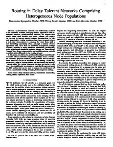
In order to measure the overhead introduced by the epidemic distribution of the MEED metric, we generated 10 topologies from the Dartmouth data with different sizes. We simulated them for one month without any traffic, and discarded the overhead in the first week. The protocol is initiated each time a connection is established, so if a scenario has more connections it will generate more overhead. To compensate for this, we normalized the overhead by dividing the total protocol bytes by the total number of connections. This gives us the average bytes of overhead that is exchanged each time we establish a connection. The average overhead with the 90% confidence interval is shown in Figure 10. The overhead appears to grow with ( 2 ), and not linearly as was predicted before. The previous result assumed that the average degree of the nodes was constant. In our scenario, nodes that share an access point form a clique, which means that adding nodes tends to increase the average node degree. The actual amount of data exchanged is still reasonable. With a network of 50 nodes, less than 10 kB is exchanged each time a connection comes up. This will take less than a tenth of a second to transmit at 802.11’s base rate of 1 Mbps. This is a tiny portion of the bandwidth, even if the contact is only up for a few seconds. With 100 nodes, the average overhead per connection is around 40 kB, which is more significant but still reasonable for high speed wireless LAN technologies. This overhead could quickly become unmanageable, which indicates that hierarchical routing would be necessary for very large deployments.
50.0k
40.0k
30.0k
20.0k
10.0k
0.0 10.0
20.0
30.0
40.0
50.0 60.0 70.0 Network Size (nodes)
80.0
90.0
Figure 10: Protocol overhead per connection
100.0
gle message, instead of one copy for every node. This is much more efficient. It also suggests that it might be possible to use the MEED metric to selectively send a small number of duplicates, in order to achieve reliable delivery at a low cost. We presented the concept of per-contact routing, where the routing tables are recomputed every time a connection is made. This permits the routing to react to topology changes and take advantage of opportunistic contacts. Indeed, the results show that this improves the latency and delivery ratio in scenarios with low bandwidth. We also showed that hop-by-hop flow control is a useful strategy for dealing with temporary buffer shortages. The most important contribution that can be made to delay-tolerant routing is to build real networks and applications. This is the only way to determine the real requirements for routing protocols. Protocols that require no configuration, like the one presented here, can facilitate this process by reducing the amount of effort required to deploy and extend these networks.
6.
REFERENCES
[1] J. Broch, D. A. Maltz, D. B. Johnson, Y.-C. Hu, and J. Jetcheva. A performance comparison of multi-hop wireless ad hoc network routing protocols. In ACM MobiCom, 1998. [2] Dartmouth College. The Dartmouth Wireless Trace Archive. http://cmc.cs.dartmouth.edu/data/. [3] J. Davis, A. Fagg, and B. Levine. Wearable computers as packet transport mechanisms in highly–partitioned ad–hoc networks. In IEEE Intl. Symp. on Wearable Computers, 2001. [4] D. S. J. De Couto, D. Aguayo, J. Bicket, and R. Morris. A high-throughput path metric for multi-hop wireless routing. In ACM MobiCom, 2003. [5] R. Draves, J. Padhye, and B. Zill. Routing in multi-radio, multi-hop wireless mesh networks. In ACM MobiCom, 2004. [6] K. Fall. A delay–tolerant network architecture for challenged internets. In ACM SIGCOMM, 2003.
[7] R. Handorean, C. Gill, and G.-C. Roman. Accommodating transient connectivity in ad hoc and mobile settings. Lecture Notes in Computer Science, 3001:305–322, March 2004. [8] B. Hull, K. Jamieson, and H. Balakrishnan. Mitigating congestion in wireless sensor networks. In ACM SenSys, 2004. [9] S. Jain, K. Fall, and R. Patra. Routing in a delay tolerant network. In ACM SIGCOMM, 2004. [10] A. Lindgren, A. Doria, and O. Schel´en. Probabilistic routing in intermittently connected networks. SIGMOBILE Mobile Computing Communications Review, 7:19–20, July 2003. [11] A. Pentland, R. Fletcher, and A. Hasson. Daknet: rethinking connectivity in developing nations. IEEE Computer, 37:78–83, 2004. [12] C. E. Perkins and P. Bhagwat. Highly dynamic destination-sequenced distance-vector routing (DSDV) for mobile computers. In ACM SIGCOMM, 1994. [13] C. E. Perkins and E. M. Royer. Ad-hoc on-demand distance vector routing. In IEEE WMCSA, 1999. [14] A. Rabagliati. Wizzy digital courier – how it works. [15] E. M. Royer and C.-K. Toh. A review of current routing protocols for ad hoc mobile wireless networks. IEEE Personal Communications, 6:46–55, 1999. [16] S. Singh, M. Woo, and C. Raghavendra. Power-aware routing in mobile ad hoc networks. In ACM MobiCom, 1998. [17] L. Song, D. Kotz, R. Jain, and X. He. Evaluating location predictors with extensive wi-fi mobility data. In IEEE INFOCOM 2004, 2004. [18] K. Tan, Q. Zhang, and W. Zhu. Shortest path routing in partially connected ad hoc networks. In IEEE GLOBECOM, 2003. [19] A. Vahdat and D. Becker. Epidemic routing for partially connected ad hoc networks. Technical Report CS-200006, Duke University, Apr 2000.