PREPROCESSING FOR DETERMINING THE DIFFICULTY OF AND SELECTING A SOLUTION STRATEGY FOR NONCONVEX OPTIMIZATION PROBLEMS R. BAKER KEARFOTT∗ AND SIRIPORN HONGTHONG† Abstract. Based originally on work of McCormick, a number of recent global optimization algorithms have relied on replacing an original nonconvex nonlinear program by convex or linear relaxations. Such linear relaxations can be generated automatically through an automatic differentiation process. This process decomposes the objective and constraints (if any) into convex and nonconvex unary and binary operations. The convex operations can be approximated arbitrarily well by appending additional constraints, while the domain must somehow be subdivided (in an overall branch and bound process or in some other local process) to handle nonconvex constraints. In general, a problem can be hard if even a single nonconvex term appears. However, certain nonconvex terms lead to easier-to-solve problems than others. In this paper, we present a symbolic preprocessing step that provides a measure of the intrinsic difficulty of a problem. Based on this step, one of two methods can be chosen to relax nonconvex terms. Key words. nonconvex optimization, global optimization, computational complexity, automatic differentiation, GlobSol, symbolic computation, linear relaxation AMS subject classifications. 90C30, 65K05, 90C26, 68Q25
1. Introduction. 1.1. The General Global Optimization Problem. Our general global optimization problem can be stated as
(1.1)
minimize ϕ(x) subject to ci (x) = 0, i = 1, . . . , m1 , gi (x) ≤ 0, i = 1, . . . , m2 , where ϕ : x → R and ci , gi : x → R, and where x ⊂ Rn is the hyperrectangle (box) defined by xi ≤ xi ≤ xi , 1 ≤ i ≤ n, where the xi and xi are constant bounds.
We will call this problem a general nonlinear programming problem, abbreviated “general NLP” or “NLP”. 1.2. Deterministic Branch and Bound Methods. In deterministic branch and bound methods for finding global minima, an initial region x(0) is adaptively subdivided into subregions x of the form in (1.1), while an upper bound ϕ to the global optimum of ϕ is maintained (say, by evaluating ϕ at a succession of feasible points). A lower bound ϕ(x) on the optimum of ϕ over the subregion x is then computed. If ϕ(x) > ϕ, then x is rejected; otherwise, other techniques are used to reduce, eliminate, or subdivide x. For a relatively early explanation of this common technique, see [13]. For more recent explanations in which convex underestimators are employed, see for example [3], [15]. For explanations focusing on validation but restricted to traditional interval arithmetic-based techniques, see [6] or [7, Ch. 5]. ∗ Department of Mathematics, University of Louisiana, U.L. Box 4-1010, Lafayette, Louisiana, 70504-1010, USA (
[email protected]). † Department of Mathematics, University of Louisiana, U.L. Box 4-1010, Lafayette, Louisiana, 70504-1010, USA (
[email protected]).
1
2
R. B. KEARFOTT AND S. HONGTHONG
The effectiveness of the above technique depends on the quality of the upper bound ϕ and the lower bound ϕ(x). The upper bound ϕ may be obtained by various techniques, such as by locating a feasible point (or local optimum) x ˇ, then evaluating ϕ at x ˇ. A naive way obtaining ϕ(x) is to simply evaluate ϕ with interval arithmetic over x, and use the lower bound of the value ϕ(x). However, ϕ(x) so obtained takes no account of the constraints, and (since the feasible portion of x, although possibly non-empty, may be much smaller than x itself) the lower bound ϕ(x) may not be sharp enough to be of use. More effective techniques appear to be those that solve coupled systems that take account of both objective and constraints. Convex and linear underestimators are used in a common variant of such techniques. 1.3. Convex Underestimators and Overestimators. Convex underestimators and overestimators are a primary tool to replace problem (1.1) by a simpler problem, the global optimum of which is less than or equal to the global optimum of (1.1). For example, if ϕ is replaced by a quadratic or piecewise linear function ϕ(`) such that ϕ(`) (x) ≤ ϕ(x) for x ∈ x, then the resulting problem has global optimum that underestimates the global optimum of (1.1). Similarly, if m1 = 0 (i.e. if there are no equality constraints) and, in addition to replacing ϕ by ϕ(q) , each gi replaced by a (`) (`) linear function gi such that gi (x) ≤ gi (x) for x ∈ x, then the resulting quadratic or linear program, termed a relaxation of (1.1), has optimum that is less than or equal to the optimum of (1.1). (If there are equality constraints, then each equality constraint can be replaced, at least in principle, by two linear inequality constraints.) 1.3.1. An Arithmetic on Underestimators and Overestimators. Constraints or objective functions that represent simple binary operations (addition, subtraction, multiplication, and division), or unary operations (standard functions such as y = ex or y = xn ) can be bounded below or above on a particular interval by linear relations. For instance, if g 1 is a linear underestimator for g1 and g 2 is a linear underestimator for g2 , then a linear underestimator for g1 + g2 is g 1 + g 2 . Thus, addition of two linear underestimators can be defined simply by addition of the corresponding linear coefficients. Similarly, if g 1 is a linear underestimator for g1 and −g 2 is a linear underestimator for −g2 , then g 1 + −g 2 is a linear underestimator for g1 − g2 . Linear underestimators for multiplication are somewhat more involved, but can similarly be obtained operationally. For convex functions such at eg , for g ∈ [a, b], a linear underestimator is the tangent line at any point c ∈ [a, b], while for concave functions g, the best possible linear underestimator is the secant line connecting (a, g(a)) (b, g(b)). If [a, b] is too wide to get sharp underestimators and overestimators, then [a, b] may be subdivided, and linear underestimators can be supplied for each subinterval. In actually generating a linear program whose solution underestimates the solution of (1.1), we replace an expression g by a new intermediate variable v for the underestimator wherever the expression g occurs; we then append the constraint v ≥ g for the linear underestimator to the set of constraints. In case multiple linear constraints are used for more accuracy, we introduce multiple variables vi and wi and corresponding multiple constraints. An arithmetic can be used to automatically compute underestimators given by expressions or computer programs. The original idea for such an arithmetic goes back to McCormick. Such an arithmetic may employ operator overloading or similar technology, such as explained, say, in [14] [7, §1.4] or in the proceedings [1], [2] or [5]. A framework for such automatic computation is given in [15, §4.1]. In such an arithmetic, given underestimators for expressions g1 and g2 , formulas are implemented
NONCONVEX OPTIMIZATION PREPROCESSING
3
for computing underestimators of g1 + g2 , g1 ∗ g2 , and g1 /g2 , as well as for computing underestimators of powers, exponentials, logarithms, and other such functions encountered in practice. Many of the ideas for such an arithmetic appear in work of McCormick [10, 11, 12]. Significant portions of the books [3] and [15] are devoted to techniques for deriving underestimators and overestimators as we have just described, and for implementing automatic computation of these. For example, [15, Chapter 3] contains techniques for computing underestimators of sums of products, and [15, Chapter 4] summarizes rules for automatic computation of underestimators, based on convex envelopes and linear underestimations. The techniques in [15] are embodied in the highly successful software package BARON. Gatzke, Tolsma, and Barton [4] have implemented automated generation of both linear underestimating techniques as in [15] and convex underestimating techniques as in [3] in their DAEPACK system. 1.4. Our View of the Process. In this work, to aid our analysis of the difficulty of particular problems, we view the process slightly differently. In particular, we first generate a list of operations (known as a code list or tape among experts in automatic differentiation), and we assign an equality constraint to each operation, leading to an equivalent expanded NLP. We may then analyze each such equality constraint in the equivalent expanded NLP to determine if we may replace the equality constraint by a “≤” constraint or a “≥” constraint, to obtain an equivalent relaxed expanded NLP. In a third step, we replace the nonlinear operations in the constraints in the equivalent relaxed expanded NLP by linear underestimators or linear overestimators. For nonlinear operations and equality constraints, both underestimators and overestimators are required, while only underestimators are required for “≤” constraints, and only overestimators are required for “≥” constraints. We call the resulting linear program a linear underestimating relaxation. This four stage scheme is diagrammed in Figure 1.1.
Original NLP equivalent
Equivalent expanded NLP equivalent
Equivalent relaxed expanded NLP just a relaxation we subdivide to make accurate
Linear relaxation Fig. 1.1. Our four stages in analyzing a linear relaxation of an NLP
For underestimators of convex operations or overestimators of concave operations, additional constraints can be appended in the linear underestimating relaxation to sharpen the approximation. However, in overestimations of convex operations or underestimations of concave operations, the linear underestimating relaxation cannot be made to more sharply underestimate the original problem by appending additional linear constraints; in these cases, in general, the domain must be subdivided, and a linear underestimating relaxation must be solved over each subproblem. In our
4
R. B. KEARFOTT AND S. HONGTHONG
procedure, we will explicitly identify those operations requiring solution of linear underestimating relaxations over subregions to obtain increased accuracy. We will also identify which (and how many) variables to subdivide to achieve the increased accuracy. The number of such variables gives the dimension of the subspace in which tessellation must occur, and thus gives a measure of how much effort needs to be expended to accurately approximate a solution. 1.5. Organization of This Work. In §2, we give a simple example that is used throughout the rest of the paper to illustrate the concepts. In §3, we define and illustrate our concept of expanded NLP and equivalent relaxed expanded NLP, and we give a theorem that shows how we may replace equality constraints by inequality constraints in the expanded NLP to obtain an equivalent relaxed expanded NLP. In §4 we give details on refining convex and concave constraints, while in §5, we describe our algorithm structure for an automatic analysis. The results of an automatic analysis appears in §6. We give conclusions and a brief outline of ongoing work in §7. 2. An Illustrative Example. Consider Example 1. Minimize ¡ ¢2 2 ϕ(x) = (x1 + x2 − 1) − x21 + x22 − 1 for x1 ∈ [−1, 1] and x2 ∈ [−1, 1]. Example 1, a small unconstrained problem except for bound constraints, is easily solved by GlobSol [8], a traditional interval branch-and-bound method. However, it is nonconvex, and can be used to illustrate underlying concepts in this work. To generate a linear relaxation of this problem, we first assign intermediate variables to intermediate operations, thus generating a code list. (This can be done within a compiler or by operator overloading.) Such a code list is seen in the second column of Table 2.1. Table 2.1 A code list, interval enclosures, and expanded NLP for Example 1.
] 1 2 3 4 5 6 7 8 9
Operation v3 ← x1 + x2 v4 ← v3 − 1 v5 ← v42 v6 ← x21 v7 ← x22 v8 ← v6 + v7 v9 ← v8 − 1 v10 ← −v92 v11 ← v5 + v10
Enclosures Constraints [−2, 2] x1 + x2 − v3 = [−3, 1] v3 − 1 − v4 = [0, 9] v42 − v5 ≤ [0, 1] v12 − v6 = [0, 1] v22 − v7 = [0, 2] v6 + v7 − v8 = [−1, 1] v8 − 1 − v9 = [−1, 0] −v92 − v10 ≤ [−1, 9] v5 + v10 − v11 ≤
0 0 0 0 0 0 0 0 0
Convexity linear linear convex both both linear linear nonconvex linear
The third column of Table 2.1 contains enclosures for the corresponding intermediate variables, based on x1 ∈ [−1, 1] and x2 ∈ [−1, 1]. (Here, we obtained these enclosures with traditional interval evaluations of the corresponding operations.) For example, the enclosure [−1, 9] in the last row represents bounds on the objective for x1 ∈ [−1, 1] and x2 ∈ [−1, 1]. We explain the fourth and fifth columns of Table 2.1 below.
NONCONVEX OPTIMIZATION PREPROCESSING
5
3. The Expanded NLP and the Equivalent Relaxed Expanded NLP. If we replace each operation in the code list by an equality constraint, we obtain an equivalent NLP, in the sense that the optimum and optimizing values of the independent variables for the resulting NLP are the same as the optimum and optimizing values of the original NLP. Definition 3.1. Given the original NLP (1.1), the expanded NLP is that NLP obtained by replacing the objective and constraints by corresponding intermediate variables for the individual operations and assigning equality constraints to the intermediate variables. In Example 1, an expanded NLP can be defined from the operations in Table 2.1, to obtain
(3.1)
minimize v11 subject to v1 + v2 − v3 = 0, v3 − 1 − v4 = 0 v42 − v5 = 0 v12 − v6 = 0 v22 − v7 = 0 v6 + v7 − v8 = 0 v8 − 1 − v9 = 0 −v92 − v10 = 0 v5 + v10 − v11 = 0 v1 ∈ [−1, 1], v2 ∈ [−1, 1].
As an intermediate step in producing a linear relaxation of the original NLP, we replace as many of the equality constraints as possible in the expanded NLP by inequality constraints subject to the resulting problem being equivalent to the original one. We do this according to the following definition and theorem. Definition 3.2. Suppose we have an expanded NLP as in Definition 3.1, and we replace as many of the equality constraints as possible in the expanded NLP by inequality constraints, according to the following rules. 1. Unless the objective consists of an independent variable only, the top-level operation ϕ = vk = f (vq , vr ) or ϕ = f (vq ) (corresponding to the bottom of the code list and evaluation of the objective) may be replaced by an inequality constraint of the form f ≤ vk . (In Table 2.1, ϕ corresponds to v11 , and f (vq , vr ) = v5 + v10 .) 2. In constrained problems, operations corresponding to ci (x) = 0 or gi (x) ≤ 0 are placed unaltered into the constraint set. For example, if gi were defined by intermediate variable vk in the code list, then the constraint vk ≤ 0 would be placed into the set of constraints. 3. (Recursive conditions) If a binary operation vi = fi (v` , vm ) or a unary operation vi = f (v` ) computes a value vi that enters only as an argument to operations vj = fj (vi , ·) or vj = fj (vi ), such that for every j, fj is monotonic in vi , then: (a) if, for those j for which fj is monotonically increasing with respect to vi , operation fj corresponds to an inequality constraint of the form fj ≤ vj , and, for those j for which fj is monotonically decreasing with respect to vi , operation fj corresponds to an inequality constraint of the form fj ≥ vj , then vi may correspond to an inequality constraint of the form f i ≤ vi .
6
R. B. KEARFOTT AND S. HONGTHONG
(b) if, for those j, for which fj is monotonically increasing with respect to vi , operation fj corresponds to an inequality constraint of the form fj ≥ vj , and, for those j for which fj is monotonically decreasing with respect to vi , operation fj corresponds to an inequality constraint of the form fj ≤ vj , then vi may correspond to an inequality constraint of the form f i ≥ vi . 4. All other operations correspond to equality constraints. Then the resulting NLP is called an equivalent relaxed expanded NLP for the original NLP (1.1). The fourth column of Table 2.1 shows the constraints corresponding to the equivalent relaxed expanded NLP corresponding to the code list in the second column of Table 2.1. Theorem 3.3. The equivalent relaxed expanded NLP of Definition 3.2 is equivalent to the expanded NLP of Definition 3.1 in the sense that: 1. The optimum of the equivalent relaxed expanded NLP is the same as the optimum of the expanded NLP. 2. The set of optimizing points of the equivalent relaxed expanded NLP contains the set of optimizing points of the expanded NLP. 3. Under a “strict monotonicity” condition described in the proof of this theorem, the sets of optimizing points of the equivalent relaxed expanded NLP and of the expanded NLP are the same. Thus, since the expanded NLP is equivalent to the original NLP, the equivalent relaxed expanded NLP is equivalent to the original NLP in the same sense. Before we prove Theorem 3.3, we use Example 1 to illustrate the process defined in Definition 3.2. Although a computer can easily label each operation as corresponding to equality or inequality by a backwards traversal of the code list, we illustrate the process with a computational graph. The computational graph corresponding to the code list in Table 2.1 appears in Figure 3.1. To label each node in the graph, we traverse the graph from the bottom up. The bottom node is labelled as “≤”. We then check the nodes immediately above nodes already checked to see if they satisfy the recursive condition 3 of Definition 3.2. Any node that fails to satisfy the recursive condition is labelled an equality constraint, and all nodes above that node in the computational graph are labelled equality constraints. Figure 3.1 illustrates the result of this process. Using Definition 3.2 (and comparing with Figure 3.1 and to the fourth column of Table 2.1), the equivalent relaxed expanded NLP for Example 1 is
(3.2)
minimize v11 subject to v1 + v2 − v3 = 0, v3 − 1 − v4 = 0 v42 − v5 ≤ 0 v12 − v6 = 0 v22 − v7 = 0 v6 + v7 − v8 = 0 v8 − 1 − v9 = 0 −v92 − v10 ≤ 0 v5 + v10 − v11 ≤ 0 v1 ∈ [−1, 1], v2 ∈ [−1, 1].
Similarly, the proof of Theorem 3.3 proceeds by induction on the nodes of the computational graph, starting at the bottom.
NONCONVEX OPTIMIZATION PREPROCESSING
x2
x1 v3 v6 ^2
7
+
must be = v4
-1
v7 ^2
< v5 ^2 v8 + must be = v 9
-1
< v10 -^2 < v11
+
Fig. 3.1. The computational graph corresponding to the code list in Table 2.1
Proof of Theorem 3.3 Assume first that the only change made to the expanded NLP is replacement of the equality constraint vfinal = f by an inequality constraint f ≤ vfinal according to rule 1, and suppose that the resulting NLP is not equivalent to the original expanded NLP. Then, since the resulting NLP is a relaxation of the original NLP, the resulting NLP must have an optimizer that is not in the feasible set of the original NLP. However, the only way this can be is if the inequality constraint f ≤ vfinal is strict. However, we may then reduce vfinal and remain in the feasible set, contradicting the assumption that vfinal represented an optimum. Now suppose that we start with a problem P that is equivalent to the expanded NLP from application of some of the rules in Definition 3.2, and suppose we obtain a new problem Pnew from P by applying rule 3a to P, that is, by replacing fi = vi by fi ≤ vi . Then, arguing as above, any optimizer of Pnew that is not an optimizer of P would need to correspond to the strict inequality fi < vi . But then, we could decrease vi until vi = fi , and each constraint in which vi occurred would remain feasible. Thus, the optimum of Pnew would have to correspond to the optimum of P, and the optimizing points of P are optimizing points of Pnew . For the stronger assertion about the optimizing sets, suppose that each fj related to any fi that occurs in rule 3a or rule 3b is either strictly increasing or strictly decreasing, and that each intermediate computation is part of either the objective or a constraint. (By this last condition, we mean that there are no “dead ends” in the computation, i.e. there are no bottom nodes in the computational graph that correspond neither to an objective nor a constraint.) Then, by decreasing vi , each fj either decreases or increases, and we can decrease or increase the corresponding vj ’s
8
R. B. KEARFOTT AND S. HONGTHONG
without affecting the feasibility of the problem. We can, in turn, decrease or increase variables depending on those vj ’s that we have so adjusted, until we adjust a variable vk upon which no other variables depend. Due to the “no dead ends” assumption, this variable vk represents, without loss of generality, either the objective value ϕ or a constraint value or g. (It cannot represent an equality constraint c = 0, since then the constraint we have relaxed could not have been replaced by an inequality in the first place.) If this variable vk represents the objective: vk ≤ ϕ, then ϕ can be decreased; this would, however, contradict the assumption that we started with an optimizer of Pnew . On the other hand, if vk represented a constraint g ≤ 0, then our adjustments will have decreased g, which means the adjusted point is further inside the interior of the feasible region of g; in turn, this means that the point must have been feasible for P, contradicting our assumption. A similar argument holds if we start with a problem P that is equivalent to the expanded NLP from application of some of the rules in Definition 3.2, and we obtain a new problem Pnew from P by applying rule 3b to P. This proves the theorem. NLP’s whose code list generates many equality constraints corresponding to nonlinear operations are more difficult to solve, in a sense to be made explicit below. This is because, to relax a nonlinear equality constraint, we obtain both a convex operation and a concave (nonconvex) operation, and a more expensive kind of branching appears necessary for nonconvex operations. The actual solution to the original NLP of Example 1 (as bounded by GlobSol) is x1 , x2 ∈ [0.269593, 0.269595], ϕ(x) ∈ [−0.51805866866, −0.51805866865]. When the approximate solver IPOPT [16] is given the equivalent relaxed expanded NLP (3.2), IPOPT happens to return values within these bounds. 4. Relaxations. We may replace each convex and nonconvex constraint in an expanded NLP by a linear relaxation. In validated computations, we also generally replace each linear equality constraint by a pair of linear inequality constraints that tightly contain the linear constraint, but take account of roundoff error in computing the coefficients. In both validated and non-validated computations, we replace each nonlinear equality constraint by a pair of inequality constraints; in this case, if the original nonlinear equality constraint was convex, we obtain both a convex and a concave constraint. Table 4.1 illustrates a possible set of relaxations for the expanded NLP of Table 2.1. In the fourth column of Table 4.1, the underestimates for the convex terms v42 , 2 x1 , and x22 correspond to the tangent lines to the operations at the midpoint of the enclosure interval; for example, the expression (4.5)2 + 9(v4 − 4.5) in the third row corresponds to the tangent line to v42 at v4 = 4.5. The nonconvex operations (−v92 , −v12 , and −v22 ) are underestimated by the secant line connecting the end points of the graph. If the expanded NLP is replaced by “minimize v11 subject to x1 ∈ [−1, 1], x2 ∈ [−1, 1], and subject to each of the constraints in column 4,” then the solution to the resulting linear program, which we call an expanded LP, underestimates the solution to the original NLP. When we gave IPOPT the expanded LP corresponding to Table 4.1, IPOPT obtained (x1 , x2 ) ≈ (0.3894, 0.3894), ϕ = −1, an underestimator that is no better than the traditional interval evaluation of the objective over the box. 4.1. Refining Convex Constraints. As explained in [15, §4.2] and elsewhere, the nonlinear convex operations can be approximated more closely in the linear relaxation by appending more constraints corresponding to additional tangent lines. For example, in the nonlinear convex operation v5 ← v42 in Example 1, in addition to the
9
NONCONVEX OPTIMIZATION PREPROCESSING Table 4.1 A linear relaxation corresponding to the expanded NLP in Table 1.
] 1 2 3 4
v3 v4 v5 v6
Operation ← x1 + x2 ← v3 − 1 ← v42 ← x21
5 v7 ← x22 6 7 8 9
v8 v9 v10 v11
← ← ← ←
v6 + v7 v8 − 1 −v92 v5 + v10
Enclosures Under/Over Estimators [−2, 2] x1 + x2 − v3 = [−3, 1] v3 − 1 − v4 = [0, 9] (4.5)2 + 9(v4 − 4.5) − v5 ≤ [0, 1] (0.5)2 + 1(v1 − 0.5) − v6 ≤ v1 − v6 ≥ [0, 1] (0.5)2 + 1(v2 − 0.5) − v7 ≤ v2 − v7 ≥ [0, 2] v6 + v7 − v8 = [−1, 1] v8 − 1 − v9 = [−1, 0] −1 − v10 ≤ [−1, 9] v5 + v10 − v11 ≤
0 0 0 0 0 0 0 0 0 0 0
Convexity linear linear convex convex nonconvex convex nonconvex linear linear nonconvex linear
constraint v5 ≥ (4.5)2 + 9(v4 − 4.5) (corresponding to the tangent line at v4 = 4.5), we may add the constraint v5 ≥ (2.25)2 + 4.5(v4 − 2.25) (corresponding to the tangent line at v4 = 2.25) and the constraint v5 ≥ (6.75)2 + 13.5(v4 − 6.75) (corresponding to the tangent line at v4 = 6.755), and any other similar tangent line. By spacing the tangent lines sufficiently close together, the corresponding convex constraint can be approximated arbitrary closely. If there were no nonconvex operations in the code list, then all convex operations could be approximated arbitrarily closely by spacing tangent lines sufficiently close together. This process involves subdivision in a single variable for each convex nonlinear constraint, so the number of constraints in a linear programming relaxation whose solution approximated the solution to the original nonlinear program to a given accuracy would seem to be, essentially, linear in the number of operations in the code list. 4.2. Refining Nonconvex Constraints. However, the relaxations for nonconvex operations cannot be refined by appending additional constraints in the same way. Two possibilities come to mind: • We may subdivide the original variables x1 and x2 to reduce the width of the enclosure for the domain of the operation corresponding to the nonconvex constraint, and thus reduce the slack in the linear underestimator for the nonconvex constraint. For example, if we bisected both x1 and x2 , for Example 1, we would obtain four sub-domains. We would obtain underestimates for the solution of the original problem over the sub-domains as underestimates to the corresponding linear relaxations; an underestimate for the original problem over the original domain would consist of the minimum of the four underestimates over the sub-domains. • Alternately, we may subdivide the domain of the operation corresponding to the nonconvex constraint directly into two or more sub-intervals (or subboxes in the case of multiplication), and form relaxations corresponding to each of these sub-intervals or sub-boxes. For example, we could subdivide v9 in Table 4.1 into [−1, 0] and [0, 1]. We then underestimate −v92 over each separate sub-interval by its secant line. If we use this secant line, along with the original bounds x1 ∈ [−1, 1], x2 ∈ [−1, 1], we obtain a relaxation of the
10
R. B. KEARFOTT AND S. HONGTHONG
problem we would get by restricting x1 and x2 to those values leading to a range of v9 in the selected subinterval (such as one of [−1, 0] or [0, 1]). Thus, the minimum of the solutions to the relaxations so obtained will be an underestimate to the solution of the original nonlinear programming problem. For example, consider, for the purpose of examining a single nonconvex operation, using the exact constraints in the expanded NLP of Table 2.1 except for that corresponding to operation 8, which we maintain as −1−v10 ≤ 0 as in Table 4.1. IPOPT gives an approximate solution (x1 , x2 ) ≈ (0.5, 0.5), ϕ ≈ −1 to this problem. We now subdivide v9 into v9 ∈ [−1, 0] and v9 ∈ [0, 1]. The relaxation of v10 ≥ −v92 over [−1, 0] corresponding to the secant line through the end points is v10 ≥ v9 . Replacing v10 ≥ −1 (valid over [−1, 1]) by this and using a corresponding bound constraint on v9 , but otherwise keeping the same convex program, IPOPT gives an approximate solution (x1 , x2 ) ≈ (0.3333, 0.3333), ϕ ≈ −0.6667. Now replacing v10 ≥ −v92 over [0, 1] by the relaxation corresponding to the secant line through the end points, namely v10 ≥ −v9 , and using a corresponding bound constraint on v9 , IPOPT gives (x1 , x2 ) ≈ (1, 0.6823), ϕ ≈ 9 × 10⁻⁵ . Thus, an underestimate for the solution to the original ª NLP, based © on these linear relaxations, is approximately min −0.6667, 9 × 10−5 = −0.6667, a tighter estimate than that obtained by solving only a single problem, but obtained by subdividing in one variable only. A similar phenomenon would be seen if, instead of using exact inequalities for the convex operations, we used a sufficient number of linear underestimators. 5. Our Preprocessing Algorithms. If there are only one or two nonconvex operations in the code list, but these nonconvex operations depend on many, if not all, of the dependent variables, then it is probably advantageous to use the second subdivision process (subdividing directly on the intermediate variables entering the nonconvex constraints). However, if there are many nonconvex constraints, all depending on the same small number of independent variables, then it is probably advantageous to do a traditional branch-and-bound within the subspace of independent variables corresponding to the nonconvex constraints. The problem will be “hard” if there are both a large number of nonconvex constraints and a large number of independent variables enter into these nonconvex constraints; otherwise, the problem is easily solvable by either branching and bounding on directly on the intermediate variables entering the few convex constraints or by branching and bounding on the few independent variables entering the nonconvex constraints. With these considerations in mind, we have structured our preprocessing algorithms in the following order. 1. We first create the code list. 2. Evaluate the code list with interval arithmetic to obtain bounds on the intermediate variables1 . 3. Using Theorem 3.3, and the bounds from Step 2 start at the bottom of the computational graph to label each node in the computational graph as corresponding to an inequality or an equality constraint. 4. Using the ranges from step 2, the labellings from step 3, and considerations from §4 (e.g. whether the function is convex or concave and whether an overestimate, underestimate, or both is required), label each node as requiring solution of problems on subdomains to obtain tighter approximations via linear programs or as requiring only appending of additional constraints to a 1 Constraint
propagation may be used at this point.
NONCONVEX OPTIMIZATION PREPROCESSING
11
single problem over the original domain. 5. For those nodes in the computational graph requiring solution of problems over subdomains, trace up the computational graph to identify upon which independent variables the result depends. Implementation of steps 3 and 3 require a case-by-case consideration of the individual operations (exponential, odd, even, or real powers, etc.). 6. Experiments. We have programmed each of the steps in §5 within the GlobSol module structure, testing our programs with Example 1 and various other small problems with certain properties. For a reasonably simple but realistic test problem, we have tried the following problem, originally from [17]. Example 2. Minimize max |fi (x)k , where
1≤i≤m
1 , 1 + ti ti = −0.5 + (i − 1)/(m − 1), 1 ≤ i ≤ m
fi (x) = x1 ex3 ti + x2 ex4 ti −
We transformed this non-smooth problem to a smooth problem with Lemar´echal’s conditions [9], to obtain: minimize v subject tofi (x) − v ≤ 0, 1 ≤ i ≤ m −fi (x) − v ≤ 0, 1 ≤ i ≤ m To test the preprocessing, we took m = 21, we took xi ∈ [−5, 5] for 1 ≤ i ≤ 4 and v ∈ [−100, 100]. The resulting output had 221 blocks, each of the form: Row. no., OP, CONSTRAINT_TYPE, NEEDS_SUBPROBLEM 1 2 3 4 5 6 7 8 9 10 11
A_X EXP X_TIMES_Y A_X EXP X_TIMES_Y X_PLUS_Y X_PLUS_B X_MINUS_Y MINUS_X X_MINUS_Y
Row number, 2 3 5 6
EQUAL_V EQUAL_V EQUAL_V EQUAL_V EQUAL_V EQUAL_V EQUAL_V EQUAL_V LESS_OR_EQ_V LESS_OR_EQ_V LESS_OR_EQ_V
F T T F T T F F F F F
corresponding independent variables: 3 1 3 4 2 4
In rows 2 and 5 (and corresponding rows in the remaining 20 blocks), the dependence was only on variables 3 and 4. In rows 3 and 6 (and corresponding rows in the remaining 20 blocks), the binary operation is a multiplication. However (cf. eg. [3,
12
R. B. KEARFOTT AND S. HONGTHONG
p. 45 ff.]), a multiplication can be both underestimated and overestimated arbitrarily closely by subdividing in only one of the two variables. Hence, this analysis reveals that we only need subdivide in variables 3 and 4 to obtain linear programs that approximate the original NLP arbitrarily closely. This can be interpreted to mean that, with branch-and-bound based on linear underestimators and overestimators, the problem is inherently two-dimensional rather than four-dimensional. In this case, the alternative would be to subdivide each of the intermediate variables corresponding to code list rows 2, 3, 5, 6, etc. Since this would result in subdivision in an 84-dimensional space, this alternative is clearly not appropriate for this problem. 7. Conclusions and Future Work. We have presented an analysis of nonlinear programming problems that leads to a way of automatically determining the difficulty of the problem. We have implemented the resulting symbolic preprocessing and have tried it on a somewhat interesting problem. Much work remains to be done. We intend to incorporate the preprocessing into an actual branch and bound algorithm. (There is an advantage to doing the preprocessing at run-time, since the labels on the computational graph depend on the ranges of the intermediate variables, and graphs may be more advantageously labelled over subdomains.) In this context, we are working on our version of linear programming formulations and solution. Finally, use of linear programs to approximate the original NLP may not work as well as other techniques, such as use of interval Newton methods, etc. for some problems. General purpose software will probably perform best if hybrid combinations of various techniques are astutely implemented. Acknowledgements. We wish to thank Sven Leyffer and Jorge Mor´e for inviting the first author to participate in the Global Optimization Theory Workshop at Argonne Laboratories, Fall, 2003. The interactions during that conference greatly clarified my thinking on the subject, and led to this work. We also wish to thank Vladik Kreinovich for pointing out various aspects of computational complexity associated with global optimization to us. REFERENCES [1] M. Berz, C. Bischof, G. Corliss, and A. Griewank. Computational Differentiation: Techniques, Applications, and Tools. SIAM, Philadelphia, 1996. [2] G. Corliss, Ch. Faure, A. Griewank, L. Hasco¨ et, and U. Naumann. Automatic Differentiation of Algorithms: From Simulation to Optimization. Springer-Verlag, New York, 2002. [3] C. A. Floudas. Deterministic Global Optimization: Theory, Algorithms and Applications. Kluwer, Dordrecht, Netherlands, 2000. [4] E. P. Gatzke, J. E. Tolsma, and P. I. Barton. Construction of convex relaxations using automated code generation techniques. Optim. Eng., 3(3):305–326, September 2002. [5] A. Griewank and G. F. Corliss. Automatic Differentiation of Algorithms: Theory, Implementation, and Application. SIAM, Philadelphia, 1991. [6] E. R. Hansen. Global Optimization Using Interval Analysis. Marcel Dekker, Inc., New York, 1992. [7] R. B. Kearfott. Rigorous Global Search: Continuous Problems. Kluwer, Dordrecht, Netherlands, 1996. [8] R. B. Kearfott. Globsol: History, composition, and advice on use. 2002. echal. Nondifferentiable optimization. In M. J. D. Powell, editor, Nonlinear Opti[9] C. Lemar´ mization 1981, pages 85–89, New York, 1982. Academic Press. [10] G. P. McCormick. Converting general nonlinear programming problems to separable nonlinear programming problems. Technical Report T-267, George Washington University, Washington, D.CThe George Washington University, 1972.
NONCONVEX OPTIMIZATION PREPROCESSING
13
[11] G. P. McCormick. Computability of global solutions to factorable nonconvex programs. Math. Prog., 10(2):147–175, April 1976. [12] G. P. McCormick. Nonlinear Programming: Theory, Algorithms, and Applications. Wiley, 1983. [13] P. M. Pardalos and J. B. Rosen. Constrained Global Optimization: Algorithms and Applications. Lecture Notes in Computer Science no. 268. Springer-Verlag, New York, 1987. [14] L. B. Rall. Automatic Differentiation: Techniques and Applications. Lecture Notes in Computer Science no. 120. Springer, Berlin, New York, etc., 1981. [15] M. Tawarmalani and N. V. Sahinidis. Convexification and Global Optimization in Continuous and Mixed-Integer Nonlinear Programming: Theory, Algorithms, Software, and Applications. Kluwer, Dordrecht, Netherlands, 2002. [16] A. W¨ achter. An Interior Point Algorithm for Large-Scale Nonlinear Optimization with Applications in Process Engineering. PhD thesis, Carnegie Mellon University, 2002. http://dynopt.cheme.cmu.edu/andreasw/thesis.pdf. [17] J. L. Zhou and A. L. Titts. An SQP algorithm for finely discretized continuous minimax problems and other minimax problems with many objective functions. SIAM J. Optim., 6(2):461–487, 1996.