QAGen: Generating Query-Aware Test Databases - Semantic Scholar

QAGen: Generating Query-Aware Test Databases ‡ ¨ Carsten Binnig† , Donald Kossmann† , Eric Lo† and M. Tamer Ozsu † ETH Zurich, Switzerland ‡ University of Waterloo, Canada † [email protected], ‡ [email protected]

size=10

ABSTRACT Today, a common methodology for testing a database management system (DBMS) is to generate a set of test databases and then execute queries on top of them. However, for DBMS testing, it would be a big advantage if we can control the input and/or the output (e.g., the cardinality) of each individual operator of a test query for a particular test case. Unfortunately, current database generators generate databases independent of queries. As a result, it is hard to guarantee that executing the test query on the generated test databases can obtain the desired (intermediate) query results that match the test case. In this paper, we propose a novel way for DBMS testing. Instead of first generating a test database and then seeing how well it matches a particular test case (or otherwise use a trialand-error approach to generate another test database), we propose to generate a query-aware database for each test case. To that end, we designed a query-aware test database generator called QAGen. In addition to the database schema and the set of basic constraints defined on the base tables, QAGen takes the query and the set of constraints defined on the query as input, and generates a queryaware test database as output. The generated database guarantees that the test query can get the desired (intermediate) query results as defined in the test case. This approach of testing facilitates a wide range of DBMS testing tasks such as testing of memory managers and testing the cardinality estimation components of query optimizers.

Categories and Subject Descriptors D.2.5 [Software Engineering]: Testing and Debugging—Testing tools; H.2.4 [Database Management]: Systems—Query processing

General Terms Algorithms, Performance, Reliability, Experimentation

Keywords Testing, Database, Symbolic Query Processing, Symbolic Database, Symbolic Execution, Query Processing

Permission to make digital or hard copies of all or part of this work for personal or classroom use is granted without fee provided that copies are not made or distributed for profit or commercial advantage and that copies bear this notice and the full citation on the first page. To copy otherwise, to republish, to post on servers or to redistribute to lists, requires prior specific permission and/or a fee. SIGMOD’07, June 11–14, 2007, Beijing, China. Copyright 2007 ACM 978-1-59593-686-8/07/0006 ...$5.00.

⋊ ⋉

S.attr6 = T.attr7 size=200

size=1500

⋊ ⋉ R.attr = S.attr 4

R

size=1000

5

size=4000

size=500

σR.attr1 :p2

T

size=20000

S size=5000

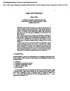
Figure 1: A test case: a query with operator constraints

1.

INTRODUCTION

When introducing a new component or technique into a DBMS, it is often necessary to validate its correctness and evaluate the relative system improvements under a wide range of test cases and workloads. Today, a common methodology is to first generate a comprehensive set of test databases and then execute many test queries over the generated databases to compare the system behavior before and after the new component is incorporated. For generating test databases, current database generation tools allow a user to define the sizes and the data characteristics (e.g., value distributions and inter/intra-table correlations) of the base tables. Examples include IBM DB2 Database Generator [2], DTM Data Generator [1], MUDD [24], or some research prototypes such as [16], [17] and [7]. Based on the generated test databases, the next step is to either create test queries manually, or stochastically generate many valid test queries by query generation tools such as RAGS [23] or QGEN [22] and execute them to test the system. Unfortunately, the current testing approach is inadequate to test individual DBMS components because very often it is necessary to control the input/output of the intermediate operators of a query during a test. For example, assume that we want to test how a newly designed memory manager in a DBMS influences the correctness and/or the performance of multi-way hash-join queries (i.e., how the per-operator memory allocation strategy affects the resulting execution plans). Figure 1 shows a sample test case (figure extracted from [8]) that is used for testing. A test case is a parametric query QP with a set of constraints defined on each operator. In Figure 1, the test query of the test case first joins a large filtered table S with a filtered table R to get a small join result. Then the small intermediate join result is joined with a filtered table T to obtain a small final result. Since the memory requirements of a hash join is determined by the size of its inputs, it would be beneficial if we can control the input/output of each individual operator in the query tree. For example, the memory allocated to 1S.attr6 =T.attr7 by the

. QP

′′′

. . QP

T1

Database 3

′′

.QP

.QP . .QP

′′′

QP ′ ′

Database 1

.QP .QP.

′

′′

Database 1

′′

QP ′′′

Database 2

T1. ... ... .. .. .. ... . . .. .. RAGS/QGEN .. . .. .queries .. . . .. ... ... .. . . . . ..

.

T2

(a) Traditional Test DB Generation

.

.

T1

T1 Database 3

... .. ... .. .. .. . . ... ..... . . ... .. .. .. ... . .. .. .. .. T2. Database 2

Database 3

Query aware test database 1

RAGS/QGEN queries

RAGS/QGEN queries

(b) Query Generation

Database 1

.

T2 Database 2

(c) Query Parameter Generation

Query aware T2 test database 2

.

(d) Query−Aware DB Generation

Figure 2: The DBMS testing problem. memory manager, can be studied by defining the output cardinality constraint on the join σ(R) 1 σ(S) and the output cardinality constraint on σ(T ) in the test case. However, although we can instruct the database engine to evaluate the test query by a specific physical evaluation plan (e.g., fixing the join order and forcing the use of hash-join as the join algorithm), there is currently no easy way to control the intermediate results of a query. [The DBMS Testing Problem] The DBMS testing problem is to guarantee that executing a test query on a test database can obtain the desired intermediate query results (e.g., output cardinalities, join distributions) that are defined by the test case. Figure 2 illustrates the problem in a conceptual way. In Figure 2(a)-(d), there are two test cases, T1 and T2 (denoted by dots); and there are three generated test database instances (denoted by squares) in Figure 2(a)-(c) respectively. In general, a good test database should cover the test cases (i.e., the database content is possible to give the desired intermediate query results for a test query when the query is executed on it). However, in traditional test database generation, the generation process does not take the queries into account. Therefore, it is hard to guarantee that executing the test query QP on the generated database can obtain the desired (intermediate) query results defined by the test case. Figure 2a shows this problem. The three generated test databases (Database 1, 2, and 3) do not cover the test case T2 at all (i.e., executing the test query of T2 on Database 1, 2, and 3 can never fulfill the constraints defined by T2 ). Furthermore, even if a test database covers a test case (e.g., Database 1 covers T1 ), it is difficult to manually find the correct parameter values P of the test query such that the resulting query matches the constraints defined by the test case. For instance, it is unlikely that instantiating the test query QP in Figure 2a with three sets of parameter values P ′ , P ′′ , P ′′′ manually can match the requirements of test case T1 . Given a test database, query generation tools such as RAGS and QGEN generate many queries in order to cover a variety of test cases. However, RAGS and QGEN were not designed for testing an individual DBMS component. To test an individual DBMS component, the desired test query is usually given by a tester (e.g., the query in Figure 1). In this situation, RAGS and QGEN would require an extremely large amount of time to generate a query that matches the test query and the requirements of the test case (see Figure 2b). In addition, RAGS and QGEN also rely on what databases they are working on or otherwise they never can generate a test query that matches the test case (e.g., T2 ). The importance of this DBMS testing problem has been pointed out by Bruno et al. [8]. Given a test database D, a parametric conjunctive query QP , and cardinality constraints C over the subexpressions of QP , they studied how to find the parameter values P of QP such that the output cardinality of each operator in QP

fulfills C. In their pioneering work, they found that their problem is N P-hard. Their approach is illustrated in Figure 2c. Given the predefined test databases (e.g., Database 1, 2, and 3), it may be possible that there are no parameter values that can let test query QP match the requirements defined by test case T2 . Furthermore, even if a test database covers a test case (e.g., Database 1), since the solution space is too large, they can only search for approximate solutions (i.e., finding parameter values that make the resulting query with cardinalities on operators close to those specified by the test case) for select-project-join queries with only single-sided predicates (e.g., p1 ≤ a or a ≤ p2 ) or double-sided predicates (e.g., p1 ≤ a ≤ p2 ) (where a is an attribute and p1 and p2 are parameter values). We observe that the test database generation process is the main culprit of ineffective DBMS testing. Currently, test databases are generated without concerning the test queries. Thus the generated databases cannot guarantee that executing the test query on them can obtain the desired (intermediate) query results defined by the test case. Therefore, the only way for meaningful testing is to do a painful trial-and-error test database generation process (e.g., generate Database 3, 2 and then 1 to find a database that matches T1 in Figure 2(a)-(c)), and execute queries generated by RAGS/QGEN, or execute test queries with parameters instantiated by [8]. [Contributions] In this paper, we address the DBMS testing problem in a different and novel way: instead of first generating a test database and then seeing if it is possible for the test query to obtain the desired query results that match the test case (otherwise use a trial-and-error approach to generate another test database), we propose to generate a specific test database tailored for each test case (see Figure 2d). To that end, we present a Query-Aware database Generator (QAGen). Given a database schema M , a parametric query QP , and a set of user-defined constraints on each query operator, QAGen directly generates a database D and query parameter values P such that executing QP with parameter values P on D guarantees that the user requirements imposed on the query operators are fulfilled. QAGen can generate test databases for a variety of complex queries such as TPC-H queries (although we will show that some rare cases are still N P-hard so that we proposed different algorithms to solve them). The test databases generated by QAGen can be used in a number of ways in DBMS testing. For example, in addition to testing the memory manager, we can use QAGen to generate a test database that guarantees the size of the intermediate join results to test the accuracy of the cardinality estimation components (e.g., histograms) inside a query optimizer by fixing the join order.1 As another example, we can use QAGen to generate a test database that guarantees the input and the output sizes (the 1 However, it is inapplicable to test the join reordering feature of a query optimizer directly because in this case the physical join ordering should not

a b t1: a1 b1 t2: a2 b2 Table R

t3: t4: t5: t6:

c c1 c2 c3 c4 Table S

d d1 d2 d3 d4

t7: t8: t9: t10:

a b=c a1 b1 b1 a1 a1 b1 b2 a2 R 1b=c S

d d1 d2 d3 d4

e f t11: e1 f1 t12: e2 f2 Table T

7. Instantiated Parameter(s)

1. Query QP, Schema M

Query Analyzer

Data Instantiator

8. Instantiated Tuple

Generated Database

σ

Figure 3: Example of pre-grouping data in symbolic query processing: (R 1b=c S) 1a=e T

Knob = ?

σ σ

T

R S

Knob = ? Knob = ?

number of groups) for an aggregation operator (GROUP-BY) in order to evaluate the performance of the aggregation algorithm under a variety of cases (e.g,. in multi-way join queries or in nested queries). Another contribution of QAGen is the novel way of defining the test database. Traditional database generators (e.g., [7, 4, 17, 1, 2]) allow constraints to be defined only on the base tables (e.g., a join distribution is defined on the base tables). As a result, a tester cannot specify operator constraints (e.g., the output cardinality of a join) in an intrinsic way. QAGen allows a user to annotate constraints on each operator and base tables directly, and thus the users can easily get a meaningful test database for a distinct test case. Sometimes it would be advantageous to add new kinds of constraints to an operator in addition to the cardinality constraint during testing. For instance, the aggregation (GROUP-BY) operator may not only need to control the output size (i.e., the number of groups), but may also need to control how to distribute the input to the predefined output groups (i.e., some groups have more tuples while others have fewer). QAGen is designed to be extensible in order to incorporate new operator constraints easily. [Roadmap] The remainder of this paper is organized as follows: Section 2 gives an overview of QAGen. Section 3 and 4 describe the algorithms used in QAGen. Section 5 presents the experimental results. Section 6 discusses related work. Section 7 contains conclusions and suggestions for future work.

2. QAGEN OVERVIEW The data generation process of QAGen consists of two phases: (1) the symbolic query processing (SQP) phase, and (2) the data instantiation phase. The goal of the symbolic query processing phase is to capture the user-defined constraints on the query into the target database. To process a query without concrete data, QAGen integrates the concept of symbolic execution [18] from software engineering into traditional query processing. Symbolic execution is a well known program verification technique, which represents values of program variables with symbolic values instead of concrete data and manipulates expressions based on those symbolic values. Borrowing this concept, QAGen first instantiates a database which contains a set of symbols instead of concrete data (thus the generated database in this phase is called a symbolic database). Figure 3 shows an example of a symbolic database with three symbolic relations R, S and T . Essentially, a symbolic relation is just a normal relational table which consists of a set of symbolic tuples. Inside each symbolic tuple, the values are represented by symbols rather than by concrete values. For example, the symbol a1 in the symbolic relation R in Figure 3 represents any value under the domain of attribute a. The formal definition of these symbolic database related terms will be given in Section 3. For the moment, let us just treat the symbolic relations as normal relations and imagine the be fixed by the tester; and the intermediate cardinalities guaranteed by QAGen may affect the optimizer that resulting in a different physical evaluation plan with different intermediate results.

3. Knob Values

2. Correct σKnob = ? knob-annotated QAGen T Knob = ? Knob = ? execution plan R S Knob = ?

Knob = ?

6. Symbolic Tuple

σ σ

5. Invoke

Symbolic Query Engine

4. Symbolic Data

Symbolic Database

Figure 4: QAGen Architecture

symbols as variables. Since the symbolic database is a generalization of relational databases and provides an abstract representation for concrete data, this gives room to QAGen to control the output of each operator of the query. The symbolic query processing phase leverages the concept of traditional query processing. First, the input query is analyzed by a query analyzer. Then, the user specifies her desired requirements on the operators of the query tree. Afterwards, the input query is executed by a symbolic query engine just like in traditional query processing; i.e., each operator is implemented as an iterator, and the data flows from the base tables up to the root of the query tree [15]. However, unlike in traditional query processing, the symbolic execution of operators deals with symbolic data rather than concrete data. Each operator manipulates the input symbolic data according to the operator’s semantics and the user-defined constraints, and incrementally imposes the constraints defined on the operators to the symbolic database. After this phase, the symbolic database is then a query-aware database that captures all requirements defined by the test case of the input query (but without concrete data). The data instantiation phase follows the symbolic query processing phase. This phase reads in tuples from the symbolic database that are prepared by the symbolic query processing phase and instantiates the symbols in the tuples by a constraint solver. The instantiated tuples are then inserted into the target database. To allow a user to define different test cases for the same query, the input query of QAGen is in the form of a relational algebra expression. For example, if the input query is a 2-way join query (σage>p1 Customer 1 Orders) 1 Lineitem, then the user can specify a distribution (e.g., a Zipf distribution) between the lineitems and the orders that join with customers with an age greater than p1 . On the other hand, if the input query is (Orders 1 Lineitem) 1 σage>p1 Customer, then the user can specify the join distribution between all orders and all lineitems. Figure 4 shows the general architecture of QAGen. It consists of the following components: a Query Analyzer, a Symbolic Query Engine, a Symbolic Database and a Data Instantiator.

2.1

Query Analyzer

At the beginning of the symbolic query processing phase, QAGen first takes a parametric query QP , the database schema M as input. The query QP is then analyzed by the query analyzer component in QAGen. The query analyzer has two functionalities: (1) Correct knob selections. It analyzes the input query and determines which knob(s) are available for each operator. A knob can be regarded as a parameter of an operator that controls the output. A basic knob that is offered by QAGen is the output cardinality

π

Available knobs

Input characteristics

Operator type

Operator

σ Equi-join

Input is pre-grouped (b) Input is not pre-grouped

Output Cardinality

(a)

on FK

Input is not pre-grouped

1) Output Cardinality 2) Join Distribution (c)

Simple aggregation

Non equi-join

x

U Single group-by attribute

Multiple group-by attributes

...

Input has tree structure

not on FK

Input is pre-grouped

Input is not Input is not Input is pre-grouped pre-grouped pre-grouped

Output Cardinality

N/A

N/A

(d)

(e)

(f)

1) Output Cardinality 2) Group Distribution (g)

Output Cardinality

(h)

1) Output Cardinality 2) Group Distribution (i)

...

...

Input has graph structure (k) Input is pre-grouped

Output Cardinality

(j)

Figure 5: Symbolic Query Processing Framework of QAGen constraint.2 This knob allows a user to control the output size of an operator. However, whether such a knob is applicable depends on the operator and its input characteristics. Figure 5 shows the knobs of each operator offered by QAGen under different cases. As an example, for a simple aggregation query SELECT MAX(a) FROM R, the cardinality constraint knob should not be available for the aggregation operator (χ), because the output cardinality is always one if R is not empty or is zero if R is empty (Figure 5 case (f)). As another example, the available knob(s) of an equi-join (1) that joins two relations (with foreign key constraint between two tables) depend on whether the input is pre-grouped or not on the join keys. If the input is pre-grouped, the equi-join can only offer the output cardinality as a single knob (Figure 5 case (d)). If the input is not pre-grouped, the user is allowed to tune the join distribution as well (Figure 5 case (c)). The input of an operator is pre-grouped on an attribute a if and only if there is at least one symbol which is not distinct in a. Consider the 2-way join query (R 1b=c S) 1a=e T on the three symbolic relations R, S, and T in Figure 3. When the symbolic relation R first joins with the symbolic relation S on attribute b and c, it is possible to specify the join distribution. For example, the first tuple t1 of R joins with the first three tuples of S (i.e., t3, t4, t5); and the last tuple t2 of R joins with the last tuple t6 of S (kind of like Zipf distribution [25]). However, after the first join, the intermediate join result of R 1 S is pre-grouped on attribute a, b and c (e.g., the symbol a1 is not distinct on the attribute a in the join result). Therefore, if this intermediate result further joins with the symbolic relation T on attribute a and e, then the distribution cannot be freely specified by a user, because if the first tuple t11 of T joins with the first tuple t7 of the intermediate results, this implies that e1 = a1 and thus t11 must join with t8 and t9 as well. The above example shows that it is necessary to analyze the query in order to offer the right knobs to the user. For this purpose, the query analyzer analyzes the input query in a bottom-up manner (i.e., starting from the input schema M ) and incrementally pre-computes the output characteristics of each operator (e.g., annotates an attribute of the output of an operator as pre-grouped if necessary). In the example, the query analyzer annotates the attributes a, b, and c as pre-grouped in the output of R 1 S. Based on this information, the query analyzer disables the join distribu2 The output cardinality of an operator can be specified as an absolute value or as a selectivity. Essentially they are equivalent.

tion knob on the next equi-join that joins with T . This step is fairly simple and is based on the work of [19] and [21], and the query analyzer can do that without analyzing the data. For space reasons, the details of this step are omitted and interested readers are referred to [6]. Nevertheless, the query analyzer essentially annotates the appropriate knob(s) to each operator according to Figure 5. As a result, the output of the query analyzer is an annotated query tree with the appropriate knob(s) on each operator. (2) Assign physical implementations to operators. As shown above, different knobs are available under different input characteristics. In general, different (combinations of) knobs of the same operator need separate implementation algorithms. Moreover, even for the same (combination of) knobs of the same operator, different implementation algorithms are conceivable (this is akin to traditional query processing where an equi-join operation can be done by hash-join or sort-merge join). Consequently, the other function of the query analyzer is to assign the correct (knob-supported) implementation to an operator. As a result, the output of the query analyzer is a knob-annotated query execution plan. Section 3 will present the implementation algorithms for each (knob-supported) operator in QAGen.

2.2

Symbolic Query Engine and Database

The symbolic query engine of QAGen is the heart of the symbolic query processing phase and it is similar to a normal query engine. It interprets the knob-annotated query execution plan given by the query analyzer. Symbolic query execution is also based on the iterator model [15]. That is, an operator reads in tuples from its child operator(s) one-by-one, processes each tuple, and returns the resulting tuple to the parent operator. Before the symbolic query engine starts execution, the user can specify the knob value(s) on the available knob(s) of each operator in the knob-annotated execution plan. It is fine for a user to fill up values for some but not all knobs. In this case, the symbolic query engine will evaluate those operators by using default knob values. Similar to traditional query processing, most of the operators in symbolic query processing can be processed in a pipelining mode but some cannot. For example, the aggregation operator with multiple group-by attributes needs to be implemented as a blocking operator, and under a special case, the equi-join operator is also a blocking operator. In these cases, the symbolic query engine materializes the intermediate results into the symbolic database if nec-

essary. In symbolic query processing, a table in a query tree is regarded as an operator. During its open() method, the table operator initializes a symbolic relation based on the input schema M and the user-defined constraints (e.g., table sizes) on the base tables. An operator evaluates the input tuples according to its own semantics. On the one hand, it imposes additional constraints to each input tuple in order to reflect the constraints defined on the operator on the data level. On the other hand, it controls its output to its parent operator so that the parent operator can work on the right tuples. As a simple example, assume the input query is a simple selection query σa≥p1 R on the symbolic relation R in Figure 3 and the user specifies the output cardinality as 1 tuple. Then, if the getNext() method of the selection operator iterator is invoked by its parent operator, the selection operator reads in tuple t1 from R, annotates a positive constraint [a1 ≥ p1 ] to the symbol a1 and returns the tuple ha1 , b1 i to its parent. When the getNext() method of the selection operator is invoked the second time, the selection operator reads in the next tuple t2 from R, annotates a negative constraint [a2 < p1 ] to the symbol a2 . However, this time it does not return this tuple to its parent, because the cardinality constraint (1 tuple) is already fulfilled. It is worth noting that sometimes a user may specify some contradicting knob values on the knob-annotated query tree given by the query analyzer. For instance, a user may specify the output cardinality of the selection in the above example as 10 tuples even if she specified the table R to have two tuples only. During runtime, when an operator cannot fulfill its output requirements even though it consumed all the input tuples, then the symbolic query engine stops processing and returns the corresponding error message to the user. By referring to the error message, the user can re-tune the knob values of the corresponding operator(s).

2.3 Data Instantiator The data instantiation phase starts after the symbolic query engine of QAGen has finished processing. The data instantiator reads in the symbolic tuples from the symbolic database and instantiates the symbols inside each symbolic tuple by a constraint solver. In QAGen, we treat the constraint solver as an external black box component which takes a constraint formula (in propositional logic) as input and returns a possible instantiation on each variable as output. For example, if the input constraint formula is 40 < a1+b1 < 100, then the constraint solver may return a1 = 55, b1 = 11 as output (or any other possible instantiation). Once the data instantiator has collected all the concrete values for a symbolic tuple, it inserts a corresponding tuple (with concrete values) into the target database.

2.4 QAGen Agenda In general, a complete QAGen system should cover all SQL operators listed in Figure 5. In this paper, we only present SQL operators that the current version of QAGen supports. They include selection (σ), projection (π), equi-join (1) and aggregation (χ). Nevertheless, these are the most commonly used operators today and they already suffice to cover 13 out of 22 complex TPC-H [4] queries. In Figure 5, the solid lines denote the operators supported by the current version of QAGen. The dotted lines show the operators or cases that the next version of QAGen should support (e.g., union (∪) and minus (−)). In addition to Figure 5, QAGen currently does not support the DISTINCT keyword and CHECK constraints imposed on UNIQUE attributes. In general, supporting new operators (e.g., union (∪)), or adding new knobs (which may depend on new input characteristics) to an operator is straightforward in QAGen. For example, adding a new knob to an operator simply means incorporating the new QAGen implementation of that oper-

ator into the symbolic query engine and then updating the query analyzer about the input characteristics that this new knob depends on.

3.

SYMBOLIC QUERY PROCESSING

In this section, we first define the data model of symbolic data and discuss how to physically store the symbolic data. Then we present the algorithms for the operators in symbolic query processing through a running example.

3.1 3.1.1

Symbolic Data Model Definitions

A symbolic relation consists of a schema and a symbolic instance. The definition of a schema is exactly the same as the classical definition of a relation schema in [11]. Let R(a1 :dom(a1 ), . . . , ai : dom(ai ), . . . , an : dom(an )) be a relation schema with n attributes; and for each attribute ai , let dom(ai ) be the domain of the attribute ai . A symbolic relation instance is a set of symbolic tuples T . Each symbolic tuple t ∈ T is an n-tuple with n symbols: hs1 , s2 , . . . , sn i. As a shorthand, the symbol si in tuple t is represented as t.ai . A symbol si is associated with a set of predicates Psi (where Psi can be empty). The value of symbol si represents any one of the values in the domain of attribute ai that satisfies all predicates in Psi . A predicate p ∈ Psi of a symbol si is a propositional formula that involves at least si , and zero or more other symbols that appear in different symbolic relation instances. Therefore, a symbol si with its predicates Psi can be represented by a conjunction of propositional logic formulas. A symbolic database is defined as a set of symbolic relations and there is a one-to-many mapping between one symbolic database and many relational databases. Finally, a symbolic relation is pre-grouped on an attribute a if and only if there is a symbol that appears twice in attribute a.

3.1.2

Data Storage

Symbolic databases are a generalization of relational databases and provide an abstract representation of concrete data. Given the close relationship between relational databases and symbolic databases, and the fact of the maturity of relational database technology, it may not pay off to re-invent the wheel and design another physical model for storing symbolic data. QAGen opts to leverage existing relational databases to implement the symbolic database concept. To that end, a natural idea for storing symbolic data would be storing the data in columns of tables, introducing a user-defined type [3] to describe the columns, and using SQL user-defined functions to implement the symbolic operations. However, symbolic operations (e.g., a join that controls the output size and distribution) are too complex to be implemented by SQL user-defined functions. As a result, we propose to store symbols (and associated predicates) in relational databases by simply using the varchar SQL data type and let the QAGen symbolic query engine operate on a relational database directly. This way, we integrate the power of various access methods brought by the relational database engine into symbolic query processing. The next interesting question is how to normalize a basic symbolic relation for efficient symbolic query processing. From the definition of a symbol, we know that a symbol may be associated with a set of predicates. For example, the symbol a1 may have a predicate [a1 ≥ p1 ] associated with it. As we will see later, most of the symbolic operations impose some predicates (from now on, we use the term predicate instead of constraints) on the symbols. Therefore, a symbol may be associated to many predicates. As a

(vii)

π

(vi)

(v)

o date

size=1

σSU M (l price) ≥:p2

c id c acctbal c id1 c acctbal1 c id2 c acctbal2 c id3 c acctbal3 c id4 c acctbal4 (i) Customer (4 tuples)

size=2

χ SU M (l price) size=8; Zipf

(iv) size=4; uniform (iii)

⋊ ⋉o id = l oid

(i) ⋊ ⋉c id = o cid Lineitem size=10

size=2 (ii)

(i) σc acctbal ≥:p1 Orders size=6

(i)

Customer size=4

c id c acctbal c id1 c acctbal1 c acctbal2 c id2 c id3 c acctbal3 c acctbal4 c id4 (i) Customer (4 tuples)

(a) Input Query Tree

o date o cid o id o id1 o date1 c id1 o id2 o date2 c id1 o id3 o date1 c id2 o id4 o date2 c id2 o id5 o date5 c id3 o id6 o date6 c id4 (ii) Orders (6 tuples)

l price l oid l id l id1 l price1 o id1 l id2 l price1 o id1 l price1 o id1 l id3 l id4 l price1 o id1 l id5 l price5 o id2 l id6 l price5 o id2 l id7 l price1 o id3 l id8 l price5 o id4 l id9 l price9 o id5 l id10 l price10 o id6 (iii) Lineitem (10 tuples) (c) Final Symbolic Database l id o id o date o cid l price l oid o id1 o date1 o cid1 l id1 l price1 l oid1 l price2 l oid2 o id2 o date2 o cid2 l id2 o id3 o date3 o cid3 l id3 l price3 l oid3 ... ... ... ... ... ... ... ... o id6 o date6 o cid6 ... (ii) Orders (6 tuples) l id10 l price10 l oid10 (iii) Lineitem (10 tuples) (b) Initial Symbolic Database

symbol acctbal1 acctbal2 acctbal3 acctbal4 l price1 l price5 aggsum1 aggsum2

c c c c

symbol

predicate [c acctbal1 ≥ p1 ] [c acctbal2 ≥ p1 ] [c acctbal3 < p1 ] [c acctbal4 < p1 ] [aggsum1 = 5 × l price1] [aggsum2 = 3 × l price5] [aggsum1 ≥ p2] [aggsum2 < p2] (iv) PTable

predicate (iv) PTable

Figure 6: Running Example result, QAGen stores the predicates of a symbol in a separate relational table called PTable. Reusing the simple selection query σa≥p1 R from Figure 3 again, the symbolic relation R can be represented by a normal table in a RDBMS named R with the schema: R(a: varchar(1024), b: varchar(1024)) and a table named PTable with the schema: PTable(symbol: varchar(1024), predicate: varchar(1024)). After the selection on R, the relational representation of the symbolic table R is: b a a1 b1 a2 b2 Table R (2 tuples)

Symbol Predicate a1 [a1 ≥ p1 ] a2 [a2 < p1 ] PTable (2 tuples)

3.2 Symbolic Query Evaluation The major difference between symbolic query execution and traditional query processing is that the input (and thus the output) of each operator is symbolic data but not concrete data. The flexibility of symbolic data allows an operator to control its internal operation and thus its output. Same as traditional processing, an operator is implemented as an iterator. Therefore the interface of an operator is the same as traditional query processing which consists of three methods: open(), getNext() and close(). During query processing, if the operator has problems due to contradicting knob values defined by the user (e.g., the output cardinality of a selection operator is bigger than its input size), that operator should return an error message to the user. For brevity, error detection during symbolic query processing is not discussed in this paper; it is straightforward to implement. In the remainder of this section, we assume that no contradicting knob values are given by the user. Next, we present the knobs and the algorithms for each operator through a running example. Unless stated otherwise, the following sub-sections only show the details of the getNext() method of each operator. All other aspects (e.g., open() and close()) are straightforward so that they are omitted for brevity. The running example is a 2-way join query which can demonstrate the details of the symbolic execution of selection, equi-join, aggregation and projection. We will also discuss some special cases of these operators. Figure 6a shows the input query tree (with all knobs and their values given). The example is based on the following simplified TPC-H schema (primary keys are underlined): Customer (c id int, c acctbal float) Orders (o id int, o date date, o cid REFERENCES Customer) Lineitem (l id int, l price float, l oid REFERENCES Orders)

3.2.1

Symbolic Execution of Table Operator

Knob: Table Size (compulsory)

In QAGen, a base table in a query tree is regarded as an operator. During the open() method, it creates a relational table in a RDBMS with the attributes specified in the input schema M . According to the designed storage model, all attributes are in the SQL data type varchar. Next, it fills up the table by creating new symbolic tuples until it reaches the defined table size. Each symbol in the newly created tuples is named using the attribute name as prefix and a unique identification number. Therefore, at the beginning of symbolic query processing, each symbol in the base table should be unique. Figure 6b shows the relational representation of the three symbolic relations Customer, Orders and Lineitem for the running example. The getNext() method of the table operator is the same as the traditional Table-Scan operator that returns a tuple to its parent or returns null (an end-of-result message) if all tuples have been returned. Note that if the same table is used multiple times in the query, then the table operator only creates and fills the base symbolic table once. Check constraints defined in the input schema M are enforced by adding a predicate to each created symbol. For example, if there is a check constraint CHECK(l price ≥ 0) on the Lineitem table, then all values in the attribute l price of the Lineitem table should have an associated tuple (e.g., hlprice1, [lprice1 ≥ 0] i) in the PTable. In the running example, there are no check constraints on all three tables. Therefore, all symbols have no predicate associated with them and thus the PTable in Figure 6b is empty. Primary keys, unique and not null constraints are enforced already because all symbols are initially unique. Foreign key constraints related to the query are taken care of by the join operator directly.

3.2.2

Symbolic Execution of Selection Operator

Knob: Output Cardinality c (optional; default value = input size)

Let I be the input and O be the output of the selection operator σ and let p be the selection predicate. The symbolic execution of the selection operator controls the size of the output as c. Depending on the input characteristics, the problem hardness and solutions are completely different. Generally, there are two different cases. Case 1: Input is not pre-grouped on the selection attribute(s) This is case (a) in Figure 5 and the selections in the running ex-

ample (Figure 6a operator (ii) and (vi)) are of this kind. This implementation is chosen by the query analyzer when the input is not pre-grouped on the selection attribute(s) and it is the usual case for most queries. In this case, the selection operator controls the output by: 1. During its getNext() method, read in a tuple t by invoking getNext() on its child operator and process with [Positive Tuple Annotation] if the output cardinality has not reached c. Else proceed to [Negative Tuple Post Processing] and then return null to its parent. 2. [Positive Tuple Annotation] If the output cardinality has not reached c, then (a) for each symbol s in t that participates in the selection predicate p, insert a corresponding tuple hs, pi to the PTable and (b) return this tuple t to its parent. 3. [Negative Tuple Post Processing] However, if the output cardinality has reached c, then fetch all the remaining tuples I − from input I. For each symbol s of tuple t in I − that participates in the selection predicate p, insert a corresponding tuple hs, ¬pi to the PTable, and repeat this step until calling getNext() on its child has no more tuples (returns null). c acctbal c id Each getNext() call on the selecc id1 c acctbal1 tion operator returns a positive tuple c id2 c acctbal2 that satisfies the selection predicate (i) Output of σ; 2 tuples p to its parent until the output cardisymbol predicate nality has been reached. Moreover, c acctbal1 [c acctbal1 ≥ p1 ] c acctbal2 [c acctbal2 ≥ p1 ] to ensure all negative tuples (i.e., tuc acctbal3 [c acctbal3 < p1 ] ples got from the child operator afc acctbal4 [c acctbal4 < p1 ] ter the output cardinality has been (ii) PTable reached) would not get some instanTable A. After selection tiated values later in the data instantiation phase that ends up passing the selection predicate, the selection operator associates the negation of predicate p to those negative tuples. In the running example, the attribute c acctbal in the selection predicate [c acctbal ≥ p1 ] of operator (ii) is not pre-grouped, because the data comes directly from the base Customer table. Since the output cardinality c of the selection operator is 2, the selection operator associates the positive predicate [c acctbal ≥ p1 ] to the symbol c acctbal1 and c acctbal2 of the first two input tuples and associates the negated predicate [c acctbal < p1 ] to the symbol c acctbal3 and c acctbal4 of the rest of the tuples. Table A(i) shows the output of the selection operator and Table A(ii) shows the content of the PTable after the selection. Case 2: Input is pre-grouped on the selection attribute(s) This is a special case of selection, and only happens when a selection is on top of a join and there is an attribute a in the selection predicate p pre-grouped. In [6], there is a proof that shows that symbolic execution of selection is N P-hard in this case. However, due to space constraints, we do not show the formal proof here. Due to its hardness and the fact that it rarely happens in practice (most selection operators can be pushed down by the user who gives the input), QAGen currently does not support this case (Figure 5 case (b)) and we plan to use approximation algorithms to solve this problem.

3.2.3 Knob:

Symbolic Execution of Equi-Join Operator Output Cardinality c (optional; default value = size of the non-distinct input)

Let R and S be the inputs, O be the output, and p be the simple equality predicate j = k where j is the (non-pregrouped) join attribute on R, and k is the join attribute on S that refers to j by a foreign key relationship. The symbolic execution of the equijoin operator ensures the join result size is c. Again, depending on whether the input is pre-grouped or not, the solutions are different, too.

Case 1: Input is not pre-grouped on the join attribute k. This is case (c) in Figure 5, where the join attribute k in the input S is not pre-grouped. In this case, it is possible to support one more knob on the equi-join operation: Knob:

Join Distribution b (optional; choices = [Uniform or Zipf]; default = Uniform)

The join distribution b defines how many tuples of input S join with each individual tuple in input R. For example, if the join distribution is uniform, then each tuple in R joins with roughly the same number of tuples in S. Both join operators in Figure 6a fall into this case. In this case, the equi-join operator (which supports both output cardinality c and distribution b) controls the output by: 1. [Distribution instantiation] During its open() method, instantiate a distribution generator D, with the size of R as domain (denoted by n), the output cardinality c as frequency, and the distribution type b as input. This distribution generator D can be the one in [16] or [9] or any statistical packages that generate n numbers m1 , m2 , . . . , mn which follow Uniform or Zipf [25] distribution with a total frequency of c. The distribution generator D is an iterator with a getNext() method. For the i-th call on the getNext() method (0 ≤ i ≤ n), it returns the expected frequency mi of the i-th number under distribution b. 2. During its getNext() call, if the output cardinality has not yet reached c, then (a) check if mi = 0 or if mi is not yet initialized, if yes, initialize mi by calling getNext on D and get a tuple r + from R (mi is the total number of tuples from S that should join with r + ). (b) Get a tuple s+ from S and decrease mi by one. (c) Join tuple r + with s+ according to [Positive Tuple Joining] below. (d) Return the joined tuple to its parent. However, during the getNext() call, if the output cardinality has reached c already, then process [Negative Tuple Joining] below, and return null to its parent. 3. [Positive Tuple Joining] If the output cardinality has not reached c, then (a) for the tuple s+ , replace the symbol s+ .k, which is the symbol of the join key attribute k of tuple s+ , by the symbol r + .j, which is the symbol of the join key attribute j of tuple r + . After this, the tuple r + and the tuple s+ should share exactly the same symbol on their join attributes. Note that the replacement of symbols in this step is done on both the tuples loaded in the memory and the related tuples in base table as well (using an SQL statement like “Update k.BaseT able Set k=r + .j WHERE k=s+ .k” to update the symbols on the base table where the join attribute k comes from). (b) Perform an equi-join on tuple r + and s+ . 4. [Negative Tuple Joining] However, if the output cardinality has reached c, then fetch all the remaining tuples S − from input S. For each tuple s− in S − , randomly look up a symbol j − on the join key j in the set minus between the base table where the join attribute j originates from and R (using an SQL statement with the MINUS keyword), replace s− .k with the symbol j − . This replacement is done on the base tables only because these tuples are not returned to the parent.

In the running example (Figure 6), after the selection on table Customer (operator ii), the next operator is a join between the selection output (Table A(i) in Section 3.2.2) and table Orders. The output cardinality c of that join (operator iii) is 4 and the join distribution is uniform. Since the input of the join on the join key o cid is not pre-grouped, the query analyzer uses the algorithm above to perform the equi-join. First, the distribution generator D generates 2 numbers (which is the size of the input R), with total frequency of 4 (output cardinality), and distribution as uniform. Assume D returns a sequence: {2, 2}. This means that the first customer c id1 should take 2 orders (o id1 and o id2) and the second customer c id2 should also take 2 orders (o id3 and o id4). As a result, the symbols o cid1 and o cid2 from the Orders table should be replaced by c id1 and the symbols o cid3 and o cid4 from the Orders table should be replaced by c id2 (Step 3 above). In order to fulfill the foreign key constraint on those tuples which do not join, Step 4 above (Negative Tuple Joining) replaces o cid5 and o cid6 by customers that did not pass through the selection filter (i.e., customer

c id3 and c id4) randomly. Table B(i) below shows the output of the join and Table B(ii) shows the updated Orders table (join keys are bold). o id o date c id=o cid c acctbal c acctbal1 o id1 o date1 c id1 c acctbal1 o id2 o date2 c id1 c acctbal2 o id3 o date3 c id2 c id2 c acctbal2 o id4 o date4 (i) Output of (σ(Customer) 1 Order); 4 tuples

o date o cid o id o id1 o date1 c id1 o id2 o date2 c id1 o id3 o date3 c id2 o id4 o date4 c id2 o id5 o date5 c id3 o id6 o date6 c id4 (ii) Orders (4 pos, 2 neg)

Table B. After Joining

After the join operation above, the next operator in the running example is another join between the above join results (Table B(i)) and the base Lineitem table (Figure 6b(iii)) in Zipf distribution. Again, the input of the join on the join key l oid of the Lineitem table is not pre-grouped and thus the above equi-join algorithm is chosen by the query analyzer. Assume that the distribution generator generates a Zipf sequence {4,2,1,1} for the four tuples in Table B(i) to join with 8 out of 10 line-items (where 8 is the user-specified output cardinality of this join operation). Therefore it produces the following output (join keys are bold): l id l price l oid c id c id1 c id1 c id1 c id1 c id1 c id1 c id2 c id2

c acctbal o date o cid l id l price o id = l oid c acctbal1 o date1 o cid1 l id1 l price1 o id1 c acctbal1 o date1 o cid1 l id2 l price2 o id1 c acctbal1 o date1 o cid1 l id3 l price3 o id1 c acctbal1 o date1 o cid1 l id4 l price4 o id1 c acctbal1 o date2 o cid1 l id5 l price5 o id2 c acctbal1 o date2 o cid1 l id6 l price6 o id2 c acctbal2 o date3 o cid2 l id7 l price7 o id3 c acctbal2 o date4 o cid2 l id8 l price8 o id4 i) Output of (σ(Customer) 1 Order) 1 Lineitem. 8 tuples

l id1 l price1 o id1 l id2 l price2 o id1 l price3 o id1 l id3 l price4 o id1 l id4 l id5 l price5 o id2 l price6 o id2 l id6 l price7 o id3 l id7 l id8 l price8 o id4 l id9 l price9 o id5 l id10 l price10 o id6 (ii) Lineitem (8 pos, 2 neg)

Table C. After 2-way join

Finally, note that if the two inputs of an equi-join are base tables (with foreign key constraint), then the output cardinality knob is disabled by the query analyzer. It is because in that case, all tuples from input R must join with input S and thus the output cardinality must be same as the size of S. Case 2: Input is pre-grouped on the join attribute k. This is a special case of equi-join when the input S is pre-grouped on the join attribute k. This sometimes happens when a preceding join introduced a distribution on k as in the example in Figure 3. In the following we show that if the input is pre-grouped on the join attribute k of an equi-join, then the problem of controlling the output cardinality (even without the join distribution) is reducible to the subset-sum problem: j k The subset-sum problem [14] j1 k1 } e.g. c1 = 5 times takes as input an integer sum c j2 k2 } e.g. c2 = 4 times j3 k3 } e.g. c3 = 2 times and a set of integers C = { c1 , ... k4 } e.g. c4 = 1 times c2 ,. . ., cm }, and outputs whether ... ... jl km } cm times there exists a subset C + ⊆ C Table R Table S such that ci ∈C+ ci = c. Consider the tables R and S in the figure on the right hand side, which are the inputs of such a join. Table R has one attribute j with l tuples all using distinct symbolic values ji (i ≤ l). Table S also defines only one attribute k and has in total ci rows. The rows in S are clustered in m groups, where the i-th group has exactly ci tuples using the same symbolic value ki (i ≤ m). We now search for a subset of those m groups in S which join with arbitrary tuples in R so that the output has the size c. Assume, we find such a subset, i.e., the symbolic values of those groups which result in the output with size c. The groups returned by such a search induce a solution for the original subset-sum problem. The subset-sum problem is a weakly N P-complete problem and there exists a pseudopolynomial algorithm which uses dynamic programming to solve it [14]. The complexity of that dynamic

P

P

P

programming algorithm is O(min(c, ci ) ∗ m), where c is the desired output cardinality, ci is the size of the i-th group in S, and m the number of different groups in S. If one of the input parameters is in binary (e.g., m is encoded as a n-bit digit and thus has the size 2n ), then the running time would be exponential in the input size. Fortunately, this means the special case of the equijoin operator (with pre-grouped input on the attribute k) is solvable in polynomial time because all the input parameters are given in unary. Since this case happens more often, we propose a dynamic programming version of equi-join for this special case. The equi-join algorithm uses dynamic programming to compute a subset of the pre-groups with a total count that matches the output cardinality. This is a blocking operator because it needs to read all the input from S first (for dynamic programming to solve the subset-sum problem). For memory reasons, all the input tuples from S are materialized in the symbolic database. One optimization for this case is that if c is equal to the input size of S, then all tuples of S must be joined with R and the invocation of the dynamic programming function can be skipped even if the data is pre-grouped. We reuse the figure above to illustrate the algorithm. Assume the join is on Table R and Table S and the join predicate is j = k. Assume Table R has three tuples (hj1i, hj2i, hj3i), and Table S has 12 tuples which are clustered into 4 groups with symbol k1, k2, k3, k4 respectively. Furthermore, assume the join on R and S is specified with an output cardinality as c = 7. The dynamic programming equi-join controls the output as follows: 1. [Dynamic programming] During its open() method, (a) materialize the input S of the join operator. (b) Extract the pre-group size (e.g. c1 = 5, c2 = 4, c3 = 2, c4 = 1) of each symbol ki by executing “Select Count(k) From S Group By k Order By Count(k) Desc” on the materialized input. (c) Invoke a dynamic programming (dp) function with the pre-group sizes and the output cardinality (e.g., c = 7) as input. The dp function (omitted here because of space) finds a subset of symbols K + in S which results in the desired total output cardinality (e.g., K + = {k1, k3} because c1 + c3 = 5 + 2 = 7 = c). If the dp function cannot find any solution, stop processing and report this problem to the user. 2. [Positive Tuple Joining] During getNext(), (a) for each symbol ki in K + , read all tuples S + from the materialized input of S which have ki as the value of attribute k. (b) Afterwards, call getNext() on R once and get a tuple r, join all tuples in S + with r by replacing the join key symbols in S + with the join key symbols in r. For example, the first five k1 symbols in S are replaced with j1 and the two k3 symbols in S are replaced with j2 (again, these replacements are done on symbols loaded in the memory and the changes are propagated to the base tables of where j and k originate from). (c) Return the joined tuples to the parent. 3. [Negative Tuple Joining] This step is the same as the Negative Tuple Joining step in the simple case (Section 3.2.3 case 1) that joins the negative tuples in input R with the negative tuples in input S.

For equi-joins, there are some more special cases such as both join keys are pre-grouped, or the join keys are bound by check constraints, etc. However, these cases rarely happen in practice and interested readers are referred to [6] for details.

3.2.4 Knob:

Symbolic Execution of Aggregation Operator Output Cardinality c (optional; default value = input size)

Let I be the input and O be the output of the aggregation operator and f be the aggregation function. The symbolic execution of the aggregation operator controls the size of the output as c.

Simple Aggregation. This is the simplest case of aggregation where there is no grouping (i.e,. no GROUP-BY keyword) defined on the query. In this

case, the query analyzer disables the output cardinality knob because the output cardinality is either 1 (not-empty input) or 0 (empty input). In SQL, there are five aggregation functions: MIN, MAX, SUM, AVG, COUNT. Due to space constraints, this section presents how to deal with SUM and MIN aggregation only. For the remaining aggregation functions, and complex aggregation functions such as MAX(l price) + AVG(l price), we refer the interested reader to [6]. Nevertheless, all of them share similar solutions for both pregrouped or non-pre-grouped input on the attribute(s) in f . The following shows the case of non-pre-grouped input: Let expr be the expression in the aggregation function f which consists of at least a non-empty set of symbols S in expr and let the size of the input I be n. 1. SUM(expr). During its getNext() method, (a) the aggregation operator consumes all n tuples from I, (b) for each symbol s in S, add a tuple hs, [aggsum = expr1 + expr2 + . . . + exprn ]i to the PTable, where expri is the corresponding expression on the i-th input tuple; and (c) return the symbolic tuple haggsumi as output. As an example, assume there is aggregation function SUM(l price) on top of the join result in Table C(i) of the previous section. Then, this operator returns one tuple haggsumi to its parent and adds 8 tuples (e.g., the 2nd inserted tuple is hl price2, [aggsum = l price1 + . . . + l price8]i) to the PTable. In fact, the above is a base case only. Except for a few special cases that we mentioned in [6], the aggregation operator could optimize the number and the size of the above predicates by inserting only one tuple hl price1, [aggsum = l price1 × 8]i to the PTable and replacing the symbols l price2, . . . , l price8 by the symbol l price1 on the base table. One reason for doing that is the size of the input may be very big, if that is the case, the extremely long predicate may exceed the SQL varchar size upper bound. Another reason is to insert fewer tuples in the PTable. And the most important reason is that the cost of of a constraint solver call is exponential to the size of the input formula in the worst case. Therefore, this optimization reduces the time of the later data instantiation phase. However, there is a trade-off: for each input tuple, the operator has to update the corresponding symbol in the base table where this symbol originates from. 2. MIN(expr). The MIN aggregation operator also uses similar predicate optimization as SUM aggregation. Again, except for a special case described in [6], during its getNext() method, (a) it regards the first expression expr1 as the minimum value and returns hexpr1 i as output; and (b) replaces the expression expri in the remaining tuples (where 2 < i ≤ n) by the second expression expr2 and inserts two tuples hexpr1 , [expr1 < expr2 ]i and hexpr2 , [expr1 < expr2 ] i to the PTable. As an example, assume there is aggregation function MIN(l price) on top of the join result in Table C(i). Then, this operator returns hl price1i as output and inserts 2 tuples to the PTable: hl price1, [l price1 < l price2]i and hl price2, [l price1 < l price2]i to the PTable. Moreover, l price3, l price4, . . . , l price8 are replaced by l price2 on the base table.

Single GROUP-BY Attribute. When the aggregation operator has one group-by attribute, the output cardinality c defines the number of output groups produced by the operator. Let g be the single grouping attribute. Again, this symbolic operation of aggregation can be divided into two cases: Case 1: Input is not pre-grouped on the grouping attribute In addition to the cardinality knob, when the symbols of the grouping attribute g in the input are not pre-grouped, it is possible to support one more knob: Knob:

Group Distribution b (optional; choices = [Uniform or Zipf]; default = Uniform)

The group distribution b defines how to distribute the input tuples into the c predefined output groups. In this case, the aggregation operator controls the output by:

1. [Distribution instantiation] During its open() method, instantiate a distribution generator D, with the size of I (denoted by n) as frequency, the output cardinality c as domain, and the distribution type b as input. The distribution generator is the same one as the one for doing equijoin (Section 3.2.3). It generates c numbers m1 , m2 , . . . , mc , and the i-th call on its getNext() method (0 ≤ i ≤ c) returns the expected frequency mi of the i-th number under distribution b (how to deal with mi = 0 is in [6]. 2. During getNext(), call D.getN ext() to get a frequency mi , fetch mi tuples (let them be Ii ) from I and execute the following steps. If there are no more tuples from its child operator, return null to its parent. 3. [Group assignment] For each tuple t in Ii , except the first tuple t′ in Ii , replace the symbol t.g, which is the symbol of the grouping attribute g of tuple t, by the symbol t′ .g. t′ .g is the symbol of the grouping attribute g of the first tuple t′ in the i-th group. Note that, the replacement of symbols in this step is done on both the tuple loaded in the memory and the related tuples in the base table as well. 4. [Aggregating] Invoke the Simple Aggregation Operator in the previous section (Section 3.2.4) with all the symbols participated in the aggregation function in Ii as input. 5. [Result Returning] Construct a new symbolic tuple ht′ .g, aggi i to its parent where aggi is the symbolic tuple returned by the Simple Aggregation Operator for the i-th group. Return the constructed tuple to its parent.

Case 2: Input is pre-grouped on the grouping attribute When the input on the grouping attribute is pre-grouped, it is understandable that this operation does not support the group distribution knob as in the above case. But if the input is pre-grouped on the grouping attribute and the output cardinality is the only specified knob, it is not a hard problem. SUM(l price) o date The aggregation operator (v) o date1 aggsum 1 in the running example (Figure aggsum 2 o date2 (i) Output of χ (2 tuples) 6) falls into this case. Referring predicate symbol to Table C(i), which is the inc acctbal1 [c acctbal1 ≥ p1 ] acctbal2 [c acctbal2 ≥ p1 ] c put of the aggregation operator c acctbal3 [c acctbal3 < p1 ] in the example. The grouping c acctbal4 [c acctbal4 < p1 ] [aggsum 1 = 5 × l price1] l price1 attribute in the example is o date, l price5 [aggsum 2 = 3 × l price5] after several joins, the data in (ii) PTable Table D. After Aggregation o date is pre-grouped into 4 pregroups (o date1 × 4; o date2 × 2; o date3 × 1; o date4 × 1). In this case, the aggregation operator controls the output by assigning tuples from the same pre-group to the same output group and each pre-group is assigned into c output groups in a round-robin fashion. In the example, the output cardinality of the aggregation operator is 2. The aggregation operator assigns the first pre-group (with o date1) which includes 4 tuples into the first output group. Then the second pre-group (with o date2) which includes 2 tuples to the second output group. When the third pre-group (with o date3) which includes 1 tuple is being assigned to the first output group (because of round-robin), the aggregation operator replaces o date3 with o date1 in order to put the 5 tuples into the same group. Similarly, the aggregation operator replaces o date4 from the input tuple with o date2. For the aggregation function, each output group gi invokes the Simple Aggregation Operator in Section 3.2.4 with all the symbols participated in the aggregation function as input, and gets a new symbol agggi as output. Finally, for each group, the operator constructs a new symbolic tuple hgi , agggi i and returns it to the parent. Table D(i) shows the output of the aggregation operator, and Table D(ii) shows the updated PTable after the aggregation in the running example. Furthermore, since the aggregation involves the attribute o date and l price, the Orders table and the Lineitem table are also updated (Figure 6c shows the updated tables).

HAVING and Single GROUP-BY Attribute. Dealing with a HAVING clause is the same as having a selection operator on top of the aggregation result (a rare exception is described in [6]). SUM(l price) o date Figure 6c shows the PTable content o date1 aggsum1 after the HAVING clause. It imposes Table E. Output of HAVING clause (1 tuple) two more constraints: [aggsum1 ≥ p2] which is the positive tuple and [aggsum2 < p2] which is the negative tuple, and it returns Table E to the parent.

Multiple GROUP-BY Attributes. When there are multiple group-by attributes, the aggregation operator depends not only on whether the input is pre-grouped, but also depends on whether the input on the group-by attributes contain a tree structure characteristic (from relations that have 1:n:m relationship) or a graph structure characteristic (from relations that have n:m:q relationship). QAGen currently supports query with tree input structure (see Figure 5). Under that case, the hardness of the problems and the algorithms are similar to the case of the single group-by attribute. For multiple group-by attributes with graph input structure or if the group-by attributes have domain constraints, they are strong N P-hard problems and QAGen currently does not support them. Due to tight space constraints, we provide the proofs in [6]. As part of our future work, we plan to use approximation algorithms to solve these hard problems.

3.2.5

Symbolic Execution of Projection Operator

SUM(l price) Symbolic execution on a projection aggsum1 operator is exactly the same as the traTable F. Output of π(1 tuple) ditional query processing, it projects the specified attributes and no additional constraints are added. As a result, the final projection operator in the running example takes in the input from Table E and ends with the result shown in Table F.

3.2.6

Symbolic Execution of Nested Query

Nested queries in symbolic query processing reuses the techniques in traditional query processing because queries can be unnested by using join operators [13]. In order to allow a user to have full control on the input, the user should give the input query in its unnested format. If the inner query and the outer query refer to the same table(s), then the query analyzer disables some knobs on operators that may allow a user to specify different constraints on the operators that work on the same table in both inner and outer query.

4. DATA INSTANTIATION The final phase of the data generation process is the data instantiation phase. The data instantiator fetches the symbolic tuples from the symbolic database and uses a constraint solver (strictly speaking, the constraint solver is the decision procedure of a model checker [10]) to instantiate concrete values for them. The constraint solver takes a propositional formula (remember that all predicates can be represented by propositional formula) as input and returns a set of concrete values for the symbols in the formula that satisfies all the input predicates and the actual data types of the symbols. If the input formula is unsatisfiable, the constraint solver returns error. Such errors, however, cannot occur in this phase because contradicting knob values are handled during symbolic query processing. A constraint solver call is an expensive operation. In the worst case, the cost of a constraint solver call is exponential to the size of the input formula [10]. As a result, the objective of the data instantiator is to minimize the number of calls to the constraint solver if possible. Indeed, the predicate size optimizations during symbolic query processing (e.g. reducing aggsum = l price1 + . . . + l price8 to

aggsum = l price1 × 8) are designed for this purpose. After the data instantiator has collected all the concrete values of a symbolic tuple, it inserts the instantiated tuple into the final test database. The details of the data instantiator are illustrated by using the running example as follows: 1. The process starts from any one of the symbolic tables, say, the Customer (4 tuples) table, until all tables are instantiated. 2. It reads in a tuple t, say hc id1, c acctbal1i, from the symbolic tables. 3. [Look up symbol-to-value cache] For each symbol s in tuple t, (a) it first looks up s in a table called SymbolValueCache in the symbolic database. The SymbolValueCache is a table in the symbolic database that stores the concrete values of the symbols that have been instantiated by the constraint solver. (b) If the symbol s has been instantiated with a concrete value, then the symbol is initialized with the same cached value and then proceeds to the next symbol in t. In Figure 6c, the symbol c id1 is the first symbol to be instantiated, thus it has no instantiated value stored in the SymbolValueCache table. However, assume later when instantiating the first two tuples of Orders table (with o id1, o id2), their o cid values will use the same value as instantiated for c id1 by looking up the SymbolValueCache. 4. [Instantiate values] Look up the predicates P of s from PTable. (a) If there are no predicates associated with s, then instantiate s by a default value that matches the actual domain of s in the input schema M . In the example, c id1 does not have any predicates associated with it (see PTable in Figure 6). Therefore, the data instantiator does not instantiate s with a constraint solver but instantiates a unique value v (because c id is a primary key), say, 1, to c id1. Afterwards, insert a tuple hs, vi (e.g., hc id1, 1i) to the SymbolValueCache. (b) However, if s has some predicates P in PTable, then compute the predicate closure of s. The predicate closure of s is computed by recursively looking up all the directly correlated or indirectly correlated predicates of s. For example, the predicate closure of l price1 is [aggsum1 = 5×l price1 AND aggsum1 ≥ p2]. Then the predicate closure (which is in the form of conjunctive propositional formula) is sent to the constraint solver (symbols exist in the SymbolValueCache are replaced by their instantiated values first). The constraint solver instantiates all symbols in the formula in a row (e.g., l price1 = 10, aggsum1 = 50, p2 = 18). For efficiency purposes, before a predicate closure is sent to the constraint solver, the data instantiator looks up another cache table called PredicateValuesCache in the symbolic database. This table caches the instantiated values of predicates. Since many predicates in the PTable essentially share the same pattern, the predicates stored in PredicateValuesCache are in the predicate pattern format. For example, the predicates [c acctbal1 ≥ p1] and [c acctbal2 ≥ p1] in Figure 6(c) share the same pattern: [c acctbal ≥ p1]. As a result, after the instantiation of the predicate [c acctbal1 ≥ p1], the data instantiator inserts an entry h[c acctbal ≥ p1], c acctbal1, p1i into the PredicateValuesCache table. When the next predicate closure [c acctbal2 ≥ p1] needs to be instantiated, the data instantiator looks up the predicate in PredicateValuesCache by its pattern; if the same predicate pattern is in PredicateValuesCache, then the data instantiator skips the instantiation of this predicate and reuses the instantiated value of c acctbal1 in the SymbolValueCache table for the symbol c acctbal2 (same for p1).

The number of constraint solver calls is minimized by the introduction of the SymbolValueCache and PredicateValuesCache tables. Experiments show that this feature is crucial or otherwise generating a 1G query-aware database takes weeks instead of hours. Finally, note that in Step 4a, if a symbol s has no predicate associated with it, the data instantiator assigns a value to s according to its domain. Except for attributes with integrity constraints (e.g., primary keys), those values can be assigned randomly or always use the same value. It is unnecessary to instantiate any extra data characteristics (e.g., distribution) for those symbols because they do not participate in the query at all (i.e., their values do not affect the query results anyway).

5. EXPERIMENTS This section shows the results of the experiments with our prototype system QAGen. QAGen was implemented in Java and installed on a Linux AMD Opteron 2.2 GHz Server with 4 GB of main memory. The symbolic database and the target database used PostgreSQL 7.4.8 and they were installed on the same machine. As a constraint solver, a publicly available constraint solver called Cogent [12] was used. We executed two sets of experiments with the following objectives: The first experiment (Section 5.1) studied the efficiency of the symbolic execution of individual operators. The second experiment (Section 5.2) studied the scalability of QAGen for generating different database sizes for different queries. In all the experiments, the generated databases 100% met the constraints defined in the input query plan.

#

1 Region 2 σ(Region) = R1 3 N ation 4 (R1 1 N ation) = R2 5 Customer 6 (R2 1 Customer) = R3 7 Orders 8 σ(Orders) = R4 9 (R3 1 R4) = R5 10 Lineitem 11 (R5 1 Lineitem) = R6 12 P art 13 σ(P art) = R7 14 (R7 1 R6) = R8 15 Supplier 16 (Supplier 1 R8) = R9 17 (N ation 1 R9) = R10 18 χ(R8) = R11 Symbolic Query Processing Data Instantiation (# Cogent-call) Total

5.1 Efficiency of Symbolic Operations The objective of this experiment is to evaluate (1) the running time of individual symbolic operators; (2) their scalability, and (3) the running time of the data instantiation phase by generating three query-aware databases in different scales (10M, 100M, and 1G). The input query was query 8 in the TPC-H benchmark [4]. Its logical query plan input to QAGen is shown in Figure 7. We chose TPC-H query 8 because it is one of the most complex queries in TPC-H with 7-way joins and aggregations. This query has various input characteristics to the operators enabling us to evaluate the performance of different operator implementations (e.g., the normal equi-join and the special case of equi-join that needs dynamic programming). The experiments were carried out in the following way: First, three benchmark databases were generated using dbgen from TPC-H benchmark. As a scaling factor, we used 10 MB, 100 MB, 1GB. Then, we executed query 8 on top of the three TPC-H databases, and collected the base table sizes and the cardinality of each intermediate result under the three scaling factors. The extracted cardinality of each intermediate result of query 8 is shown in Table 1 (Output-size) columns. Next, we generated three TPCHquery-8-aware databases with the collected base table sizes and output cardinalities as input and measured the efficiency of QAGen for generating databases that produced the same cardinality results. For this experiment, the join distribution was uniform. Table 1 shows the cost breakdown of generating query-aware databases for TPC-H query 8 in detail. QAGen only took about 10 minutes for generating a 10MB query-aware database. The symbolic query processing phase was fast and scaled linearly. It took about 1 minute for 10MB and less than 3 hours for 1G database. The longest SQP operations were the initialization of the big symbolic table Lineitem (Line 10 in Table 1), and the join between the intermediate result R5 and Lineitem (Line 11). That join needed long time because it accessed the large Lineitem table frequently to update the symbolic values of the join attributes. In query 8, the input was pre-grouped on the last join (line 17 in Table 1 and operator (17) in Figure 7). However, the dynamic programming equi-join finished quickly because the input and output sizes were not big. Table 1 also shows that the symbolic execution of each individual operator scaled well. The data instantiation phase dominated the whole data generation process. It took about 9 minutes to instantiate a 10M query 8 aware database and about 17 hours to instantiate a 1G query 8 aware database. Nevertheless, about 40% of time were the overhead of reading symbolic tuples and inserting concrete tuples (not shown in the Table). In the experiments, the number of constraint solver (cogent) calls was small – there were only 14 calls for 3 scaling factors. The number of calls was constant because the data

Symbolic operation

size = 10M Output-size Time 5 < 1s 1 < 1s 25 < 1s 5 < 1s 1.5k < 1s 0.3k 1s 15.0k 4s 4.5k 8s 0.9k 3s 60.0k 26s 3.6k 34s 2.0k < 1s 12 1s 29 3s 0.1k < 1s 29 < 1s 29 < 1s 2 < 1s 01m : 20s 09m : 31s (14) 10m : 51s

size = 100M Output-size Time 5 < 1s 1 < 1s 25 < 1s 5 < 1s 15.0k 5s 3.0k 7s 150.0k 45s 45.0k 67s 9.0k 22s 600.5k 237s 35.7k 348s 20.0k 5s 147 8s 282 27s 1k < 1s 282 1s 282 < 1s 2 1s 12m : 53s 96m : 03s (14) 108m : 56s

size = 1G Output-size Time 5 < 1s 1 < 1s 25 < 1s 5 < 1s 150k 49s 299.5k 75s 1.5m 553s 457.2k 709s 91.2k 277s 6001.2k 2629s 365.1k 4694s 200k 60s 1451 72s 2603 533s 10k 3s 2603 6s 2603 3s 2 10s 161m : 13s 1062m : 54s (14) 1224m : 07s

Table 1: QAGen Execution Time for TPC-H Query 8 Query 1

2

3

10

12

Phase SQP DI Total SQP DI Total SQP DI Total SQP DI Total SQP DI Total

10M 02m:40s 07m:42s 10m:22s 00m:09s 02m:27s 02m:36s 01m:35s 09m:34s 11m:09s 01m:16s 09m:42s 10m:58s 02m:11s 12m:01s 14m:12s

100M 26m:45s 78m:35s 105m:10s 01m:32s 24m:55s 26m:27s 16m:18s 97m:07s 113m:25s 12m:56s 98m:13s 111m:09s 21m:32s 123m:04s 144m:36s

1G 321m:27s 844m:52s 1166m:19s 16m:47s 249m:50s 256m:37s 185m:21s 1016m:59s 1202m:20s 156m:22s 1107m:10s 1263m:32s 244m:07s 1387m:27s 1631m:34s

Table 2: QAGen Scalability

instantiator cached the pattern of the predicates but not the concrete predicates. We indeed repeated the same experiment by turning off the caching feature of QAGen, but it ended up that the data instantiation phase for a 1G database could not finish within 2 weeks because the constraint solver took a lot of time. It proved that the predicate optimization in SQP and the caching in the data instantiator work effectively.

5.2

Scalability of QAGen

The second experiment is to evaluate the scalability of QAGen for generating a variety of query-aware test databases. Currently, QAGen supports 13 out of 22 TPC-H queries. It does not support some queries because those queries either fall into the special cases of QAGen (e.g., query 5 (Q5) falls into the special case of selection in Section 3.2.2 case 2); or because some of them use non-equi-join (e.g., Q16, Q22). Nevertheless, we generated queryaware databases for the rest of the queries in three different scaling factors 10M, 100M, and 1G. We only present part of the detailed results (Q1, Q2, Q3, Q10, Q12) here because of space constraints (see Table 3). For all 13 queries, experimental results show that the data instantiation (DI) phase was still the time dominating phase and that the symbolic query processing (SQP) phase was fast. In addition, experimental results show that both phases scaled well for all 13 TPC-H queries.

6.

RELATED WORK The closest related work in DBMS testing is the work of [8]

Acknowledgment

R11 (18)

The authors would like to thank Wing-Kai Hon and Marc Nunkesser for their insightful comments on this project.

R10 (17)

R9 (16)

N

R8 (14)

S (15)

R6

R7

σ (13)

(11)

R5 (10)

(9)

R3

L

P (12)

R4

σ (8)

(6)

R2 (4)

(5)

C

O (7)

R1 (2)

σ

(1)

R

(3)

N

Figure 7: Input Logical Query Plan (C=Customer, N =Nation, L=Lineitem, O=Orders, P =Part, R=Region, S=Supplier) which studied how to generate query parameters for test queries with the test databases given. However, existing database generation tools such as [2, 1, 16, 17, 7] were designed to generate general-purpose test databases without concerning the test queries, and thus the generated databases cannot guarantee they cover specific test cases. As a consequence, [8] can hardly find a good database to work on and eventually only a limited subset of SQL is supported. QAGen extends symbolic execution [18] and proposes the concept of symbolic query processing (SQP) to generate query-aware databases. SQP is related to constraint databases (e.g., [20]); however, constraint databases focus on constraints that represent infinite concrete data (e.g., spatial-temporal data) whereas SQP works on finite but abstract data. Recently, [5] also studied the problem of query-aware test database generation. In particular, [5] proposed the concept of reverse query processing which takes an application query and the corresponding query result as input, and processes the query reversely in order to generate a database that can return the given query result. The focus of reverse query processing is to generate minimal size test databases for functional testing of database applications, rather than testing the DBMS itself.

7. CONCLUSIONS AND FUTURE WORK This work presented QAGen, a system which generates tailormade test databases for different DBMS test cases. QAGen is based on symbolic query processing, a technique that combines traditional query processing and symbolic execution from software engineering. It could be shown that QAGen is able to generate query-aware databases for complex queries and it scales linearly. As described in our agenda (Section 2.4), one of our most important avenues for future work is to support more operators and to support more special cases in QAGen. Another important piece of future work is to exploit the possibility of generate a single database for different query plans of the same test query to test the plan selection feature of the query optimizer. Finally, we believe the work of SQP can be integrated with traditional symbolic execution so as to extend program verification and test case generation techniques to support database applications.

8.

REFERENCES

[1] DTM Data Generator. http://www.sqledit.com/dg/. [2] IBM DB2 Test Database Generator. http://www306.ibm.com/software/data/db2imstools/db2tools/db2tdbg/. [3] International Organization for Standardization (ISO). Information Technology-Database Language SQL, 1999. [4] TPC benchmark H. http://www.tpc.org/tpch. [5] C. Binnig, D. Kossmann, and E. Lo. Reverse query processing. In ICDE, 2007. ¨ [6] C. Binnig, D. Kossmann, E. Lo, and M. T. Ozsu. QAGen: Generating Query-Aware Test Databases. ETH Zurich Technical Report, 2007. [7] N. Bruno and S. Chaudhuri. Flexible database generators. In VLDB, pages 1097–1107, 2005. [8] N. Bruno, S. Chaudhuri, and D. Thomas. Generating Queries with Cardinality Constraints for DBMS Testing. TKDE, 2006. [9] S. Chaudhuri and V. Narasayya. TPC-D data generation with skew. [10] E. M. Clarke, O. Grumberg, and D. A. Peled. Model Checking. 2000. [11] E. F. Codd. A relational model of data for large shared data banks. Commun. ACM, 13(6):377–387, 1970. [12] B. Cook, D. Kroening, and N. Sharygina. Cogent: Accurate theorem proving for program verification. In CAV, pages 296–300, 2005. [13] R. A. Ganski and H. K. T. Wong. Optimization of nested SQL queries revisited. In SIGMOD, pages 23–33, 1987. [14] M. R. Garey and D. S. Johnson. Computers and Intractability; A Guide to the Theory of NP-Completeness. 1990. [15] G. Graefe. Query evaluation techniques for large databases. ACM Comput. Surv., 25(2):73–170, 1993. [16] J. Gray, P. Sundaresan, S. Englert, K. Baclawski, and P. J. Weinberger. Quickly generating billion-record synthetic databases. In SIGMOD, pages 243–252, 1994. [17] K. Houkjær, K. Torp, and R. Wind. Simple and realistic data generation. In VLDB, pages 1243–1246, 2006. [18] J. C. King. Symbolic execution and program testing. Commun. ACM, 19(7):385–394, 1976. [19] A. Klug. Calculating constraints on relational expression. TODS, 5(3):260–290, 1980. [20] B. Kuijpers. Introduction to constraint databases. SIGMOD Rec., 31(3):35–36, 2002. [21] G. N. Paulley and P.-A. Larson. Exploiting uniqueness in query optimization. In ICDE, pages 68–79, 1994. [22] M. Poess and J. M. Stephens. Generating thousand benchmark queries in seconds. In VLDB, pages 1045–1053, 2004. [23] D. R. Slutz. Massive Stochastic Testing of SQL. In VLDB, pages 618–622, 1998. [24] J. M. Stephens and M. Poess. Mudd: a multi-dimensional data generator. In WOSP, pages 104–109, 2004. [25] G. Zipf. Human Behaviour and the Principle of Least Effort. 1949.