Parameter Estimation in Coding Chains. Marco Visentini-Scarzanella1. Marco
Tagliasacchi2. Pier Luigi Dragotti1. 1. Communications and Signal Processing ...
Quantisation Invariants for Transform Parameter Estimation in Coding Chains Marco Visentini-Scarzanella1
Marco Tagliasacchi2
Pier Luigi Dragotti1
1
Communications and Signal Processing Group Imperial College London, London, United Kingdom. 2 Dipartimento di Elettronica e Informazione Politecnico di Milano, Milan, Italy. Abstract We examine the case of a signal going through a processing chain consisting of two transform coding stages, with the aim of recovering the unknown parameters of the first encoder. Through number theoretical considerations, we identify a lattice of quantisation invariant points, whose coordinates are not affected by the double quantisation and whose parameters are closely related to the unknown transform. The conditions for this lattice to exist are then discussed, and its uniqueness properties analysed. Finally, an algorithmic procedure to recover the invariants from a sparse set of points is shown together with numerical results.
1
Introduction
The effectiveness and computational simplicity of transform coding [1] has made it the de facto lossy compression standard for virtually all multimedia information that is shared on the web and stored in offline systems. This includes JPEG and JPEG2000 compression standards [2, 3] and H.26x compression algorithms [4]. Given the centrality of transform coding in widespread media objects, the information forensics community has turned its attention to the problem of uncovering the past history of objects that have been processed with coding chains, with applications including tampering detection, digital restoration and no-reference quality assessment. Some of the coding chains considered include single [5], double [6] or multiple [7] JPEG compression. Similar techniques have been also applied to video signals [8]. All of the works mentioned require knowledge of the specific coding standard employed. It is therefore important to develop methods to retrieve the transform parameters in a generic context, i.e. without any knowledge of the specific standard in use. Our work is similar in spirit to [9], where the authors present a method for recovering the transform parameters from a set of N observed points after single transform coding. Many signals such as images however, are often compressed more than once. In this work, we focus on the case of a signal x with a more complex ‘history’ of two cascaded transform coding stages, consisting of the orthogonal transforms T1 , T2 with uniform quantisation step sizes ∆1 and ∆2 respectively. 1
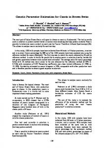
Figure 1: Double quantisation pipeline. The original signal x is encoded and decoded by an unknown orthogonal transform T1 with uniform quantisation step ∆1 . The observed signal is re-encoded by a second transform T2 (known) with quantisation step ∆2 Following the pipeline shown in Figure 1, the signal x first undergoes a transform T1 , where T1 is an orthogonal matrix with det (T1 ) = 1, yielding the rotated signal xr . This is then quantised into xq by a uniform quantiser with step ∆1 , and decoded into y by inverting the initial transform T1 . The decoded signal y is encoded a second time by a system with known parameters T2 and ∆2 , at which the quantised output yq is observed. Our contribution is to study the effect of the above coding chain on the signal structure in the case where only the parameters of the second coder are known. In particular, the aim of this work is to give an answer to the question of whether it is possible to uncover the individual coding operations in the context of a double encoding chain: starting from the final output yq , we aim to determine the conditions under which it is possible to navigate back up the signal’s history to the first coding stage and determine the first encoder’s exact transform parameters. In the following sections, we analyse the requirements for the input signal and the two encoders in order to be able to recover the parameters of the first system. Whenever such requirements are satisfied, it is then possible to follow an algorithmic procedure to exactly recover the unknown parameters, as outlined in Section 4. Results are then presented in Section 5.
2
Effects of double quantisation
In this section, we examine the effect of the second quantisation on the spatial layout of the samples. Since the quantisation is performed independently along each dimension, the signal xq observed after the first quantisation consists of samples from an upright square lattice. When considering the combined orthogonal transform T1−1 T2 , the signal yr will still consist of samples from a regular lattice rotated by the net transformation angle θ. At this stage in the processing chain, it would be still feasible to retrieve the transform parameters using, for example, the method in [9]. However, the second quantisation breaks the regularity of the original structure in
2
a nontrivial fashion, making it difficult to recover the parameters using basis reduction methods, especially if the second quantisation step is comparable in size to the first. Some examples of doubly quantised signals are shown in Figure 2(b), where ∆2 = ∆21 . 10
10
6
4
4
4
2
2 y
0
0
2
y
2
2 y2
8
6
6
−2
−2
−4
−6
−6
−6
−8
−8 −5
0 y1
5
−10 −10
10
0 −2
−4
−4
−10 −10
10
8
8
−8 −5
0 y1
5
−10 −10
10
−5
0 y1
5
10
−5
0 y
5
10
(a) 10
10
6
4
4
4
2
2
0
y
0
q2
y
q2
2 yq2
8
6
6
−2
−2
−4
−6
−6
−6
−8
−8 −5
0 y
5
10
−10 −10
0 −2
−4
−4
−10 −10
10
8
8
−8 −5
0 y
q1
q1
5
10
−10 −10
q1
(b)
(c)
Figure 2: (a) The signal yr after single quantisation and overall rotation by an angle θ is a regular lattice, here shown (from left to right) for θ = ( π4 , π6 , π9 ). (b) The signal yq after the second quantisation. (c) Fourier transform of (b). Despite the radical effect on the signal’s spatial layout, the spectrum of the original signal before the second quantisation is roughly preserved. Figure 2(c) shows the 2D-FT of the signals in (b), and the lattice structure of its peaks. It is worth noting how, despite the ‘noise’ introduced by the second quantisation making the signal’s structure deviate from a lattice, the peaks in the Fourier domain still form a lattice whose orientation roughly reflects the net rotation angle θ. A 2D lattice rotated by an orthogonal matrix T maintains its structure during the Fourier transform, i.e.:
3
X2 (M t1 , N t1 ) F
∞ X
=
∞ X
T δ(t1 − mM, t2 − nN )
m=−∞ n=−∞
∞ ∞ X X m n 1 T −1 δ f1 − , f2 − {X2 (M t1 , N t1 )} = det (T ) m=−∞ n=−∞ M N
�
�.
(1)
However, while the Fourier peak orientation can provide information about θ despite the double quantisation, this still produces approximate results. The resolution is low, affecting the precision of the measurements especially for small angles, and most of the quantisation bins would have to be populated since for the transform relationship in (1) to be maintained a complete lattice as the input signal is required. In the next section, we identify invariant points within doubly quantised signals that enable the exact recovery of the transform parameters, and we analyse the conditions for their existence.
3
Quantisation invariants
Quantisation is intimately related to modular arithmetic; the coordinates of the doubly quantised signal can be expressed in terms of the samples of the upright lattice indices xq as: "
#
"
$
∆1 cos θ − sin θ yq1 = ∆2 yq2 ∆2 sin θ cos θ
#"
xq1 xq2
#%
,
(2)
where the rotated points yr before the second quantiser correspond to: "
#
"
yr1 cos θ − sin θ = ∆1 yr2 sin θ cos θ
#"
#
xq1 . xq2
(3)
After the second quantisation, the coordinates of every sample of yq will be quantised to multiples of the second quantisation step ∆2 , i.e. by substituting Eq. (3) into (2): �
mod (∆2
yr(1,2) � , ∆2 ) = 0 ∆2
(4)
In order to characterise the periodicity of the points’ structure in the (yq1 , yq2 ) space, we are interested in the relationship between the rotated coordinates yr = (yr1 , yr2 ) and their remainder r = (r1 , r2 ) after quantisation with step ∆2 . If we consider a generic rotated point yr and all its multiples with coordinates (ayr1 , byr2 ), we can express the flooring effect introduced by quantisation as: (
mod (a∆1 (xq1 cos θ − xq2 sin θ), ∆2 ) = r1 , (a, b) ∈ Z. mod (b∆1 (xq1 sin θ + xq2 cos θ), ∆2 ) = r2
(5)
We are interested in identifying sets of points that share the same quantisation remainder r: if a relationship between the spacing and orientation of one such series 4
in (5) and the transform parameters can be established, it might be possible to obtain the unknown values directly from a subset of the samples after second quantisation. In particular we concentrate on the case where (r1 , r2 ) = 0. In this case, the points yq = yr , are therefore invariant to the second quantisation. This means that if there are cases in which it is possible to have points that do not suffer from the flooring effect during quantisation, then these points will form a regular sequence as the solution of (5) whose characteristics depend on the unknown transform parameters. Concerning the other cases where (r1 , r2 ) 6= 0, we make use of basic number theoretical considerations. From the Linear Congruence theorem [10], we know that there are solutions to Eq. (5) if and only if the following relationships are satisfied: (
gcd (∆1 (xq1 cos θ − xq2 sin θ), ∆2 )|r1 , gcd (∆1 (xq1 sin θ + xq2 cos θ), ∆2 )|r2 .
(6)
In Eq. (6) above, gcd (A, B) is the greatest common divisor operator between two terms, while A|B indicates that term A divides term B. Given a sequence of samples consisting of a generic point with coordinates (xq1 , xq2 ) rotated by an angle θ and all its multiples with coordinates (ayr1 , byr2 ), the divisibility requirements in (6) are satisfied either if the rotated coordinates and the second quantisation step are coprime, or if the remainders are zero, i.e. the points in yr are already exact multiples of the second quantisation step before the quantisation operation. Guaranteeing that the rotated coordinates and the second quantisation step are coprime would be difficult, since there is no reason for the step size to be prime. Moreover, the fact that θ is a generic angle means that generally the pairs (yr1 , ∆2 ), (yr2 , ∆2 ) would be incommensurable and the notion of greatest common divisor ceases to make sense. Hence, we focus on the first case and characterise the set of points invariant to double quantisation. In the next section, we characterise the set of invariant points as a sublattice whose characteristics are related to the first transformation, and we analyse the conditions under which it is possible to recover the transformation history.
3.1
Pythagorean triples
In a practical system, it is unlikely for the steps to be irrational numbers. As a consequence, the condition in Eq. (6) implies that as a necessary condition for it to be true the points yr must be rational numbers. Given that these points are the result of a rotation by an arbitrary angle θ, which will generally result in irrational coordinates, some constraint must be placed on the range of angles that can satisfy (6). In general, the only angles that generate a rational result in a trigonometric function are those generated by Pythagorean triples [11]. Pythagorean triples are sets of three positive integers (a, b, c) representing the sides of a right-angle triangle satisfying a2 + b2 = c2 , (a, b, c) ∈ N+ ,
5
(7)
where N+ is the set of positive integers. A generating formula for all primitive Pythagorean triples which results in all primitive right-angled triangles with integer sides is given by Euclid’s formula [11]: a = u2 − v 2 , b = 2uv, c = u2 + v 2 , (u, v) ∈ N+ .
(8)
From the definition, it is also possible to prove that there are infinitely many Pythagorean triples corresponding to as many different angles [11]. Additionally, in order to generate primitive Pythagorean triples, the integers u and v have to satisfy the following properties: gcd (u, v)
=1 (u − v) = 1 u>v
mod 2 .
(9)
∆0
1 We also define ∆10 to be the reduced form of the ∆ so that ∆01 , ∆02 have no common ∆2 2 factors. Having introduced the notions of ∆01 , ∆02 and Pythagorean triples for rational trigonometric functions, we can now prove the following theorem about the lattice of invariants’ structure.
Theorem 1. Given a rotation angle θ representable by a Pythagorean triple generated by the√integer tuple (u, v), there exists a lattice of invariants with step size µ = ∆2 ∆01 u2 + v 2 and orientation φ = 2θ . Proof. Given the generating equation for Pythagorean triples and substituting in place of the trigonometric functions, the doubly quantised points in Eq. (2) can be represented as: ∆01 = ∆2 ∆02 $ ∆01 y = ∆ q2 2 ∆02 $
yq1
!%
2uv u2 − v 2 xq1 − 2 xq2 , 2 2 u +v u + v2 !% u2 − v 2 2uv xq1 + 2 xq2 . u2 + v 2 u + v2
(10)
When substituting for (xq1 , xq2 ) a point with coordinates α(u, −v), where u and v are the generators of the Pythagorean triple and α is an integer, Eq. (10) yields quantisation invariant points, i.e. points with integer coordinates before the second quantisation: ∆01 = ∆2 ∆02 $ ∆01 yq2 = ∆2 ∆02 yq1
$
!%
u2 − v 2 2uv αu + 2 αv = α0 u∆2 ∆01 , 2 2 2 u +v u +v !% 2uv u2 − v 2 αu − 2 αv = α0 v∆2 ∆01 , u2 + v 2 u + v2
(11)
where α is such that ∆02 |α and α0 = ∆α0 . Similarly, by substituting α(v, −u) one obtains 2 α0 (v, u)∆2 ∆01 after quantisation. Hence, all invariant points together create an oriented rectangular lattice Λ with orthogonal basis vectors (v1 , v2 ) = ∆2 ∆01 ([u, v], [v, u]). The lattice step size µ stated in our theorem follows directly from the basis vectors. 6
Concerning the orientation angle φ = tan−1 uv of the lattice of invariants, this is related to the angle θ as initially stated in our theorem, since: 1− v2 tan (φ) = 2 = u 1+ 2
u2 −v 2 u2 +v 2 u2 −v 2 u2 +v 2
=
1 − cos(θ) θ ⇒φ= , 1 + cos(θ) 2
(12)
which concludes our proof. Summarising, in this section we have demonstrated that if the rotation angle can be generated by a Pythagorean triple, the doubly quantised points will contain an invariant lattice whose orientation and step size can be used to recover exactly the original transform. What remains to be proven is that the invariant lattice found in (11) is not a sublattice of another invariant lattice as well as the only possible invariant lattice that can be found. This will be shown in the next section.
3.2
Uniqueness of invariant lattices
We can test the existence of alternative invariant points by assuming that instead of a point with coordinates proportional to the Pythagorean triple generators as found in Eq. (11), we have a generic point xq = (xq1 , xq2 ). In this case, the point will be invariant to quantisation if the denominator in Eq. (10) is cancelled out, i.e.: (
(u2 − v 2 )xq1 − (2uv)xq2 = t1 (u2 + v 2 ) , (t1 , t2 ) ∈ Z. (2uv)xq1 + (u2 − v 2 )xq2 = t2 (u2 + v 2 )
(13)
The system above implies that the left hand sides must have some common factors (t1 , t2 ) that can be factored out. But since gcd (u, v) = 1 by the properties of Pythagorean triples generators in (9), then the common factors must be represented by the coordinates (xq1 , xq2 ). Therefore, there is a limited number of possibilities of what these common factors can be. In particular, xq1 can be of any form from the set {2, α1 xq2 , α1 u, α1 v}, where α1 is an integer. Similarly xq2 can be of any form from the set {2, α2 xq2 , α2 u, α2 v}, α2 ∈ Z. If we assume that xq1 = α1 xq2 , then t1 = t2 = xq2 and by simplifying and rearranging the two equations in the system, we have: (
α1 (u2 − v 2 ) − 2uv = u2 + v 2 , α1 u = v.
(14)
Taking under consideration the second equation in the system, we have that αu = v. However, from the properties of (u, v) in (9), u and v do not have any common factors, hence we have a contradiction and xq1 6= α1 xq2 . By a similar argument, xq2 6= α1 xq1 . Therefore, gcd (xq1 , xq2 ) = 1. Considering the possibility that xq1 = 2, we notice that in order to have a common factor in both equations in the system then either xq2 = 2, which would not be possible since gcd (xq1 , xq2 ) = 1, or xq2 ∈ {α2 u, α2 v}. But if this were the case, then xq1 = 2 is just a special instance of xq1 = α1 u, and xq2 = α2 v. Therefore, the only possible solutions are that (xq1 , xq2 ) ∈ {α2 u, α2 v}, with the additional constraint that 7
if xq1 = α1 u then xq2 = α2 v and vice versa. We now proceed to verify that the solution found in (11) represents the fundamental lattice and not a sublattice of the real solution. Substituting (α1 u, α2 v) for (xq1 , xq2 ) in (13) and factorising: (
u(α1 u2 − α1 v 2 − 2α2 v 2 ) = t1 (u2 + v 2 ), v(α2 u2 − α2 v 2 + 2α1 u2 ) = t2 (u2 + v 2 ).
(15)
Since (u, v) are the only elements that can be factored out, it follows that t1 = u and t2 = v respectively. Combining the two equations and simplifying we have a relationship linking α1 and α2 : − α1 (u2 + v 2 ) = α2 (u2 + v 2 ) ⇒ α1 = −α2
(16)
Since α1 and α2 are integers by definition, it follows that the lattice found in (11) is the fundamental lattice, where (α1 , α2 ) ∈ {1, −1}. Given the uniqueness property of the lattice of invariants, we present a simple algorithmic procedure to test the observed samples and check automatically their conformity to the lattice. This procedure is described in the next section.
4
Algorithmic solutions
Based on the characteristics of the lattice of invariants Λ and its uniqueness highlighted in the previous section, we devise some simple criteria that can be used to test whether one of the observed samples in yq belongs to Λ. While in this section we assume knowledge of the first quantisation step size ∆1 , it is possible to retrieve it with existing methods such as [12]. We start with a candidate set containing all observed points. Since all invariant points lie on Λ, it follows that they lie on concentric circumferences centred at the origin and with radii multiples of ∆2 ∆01 . Therefore, it is possible to remove from the set of invariant candidates all points whose squared norm is not divisible by (∆2 ∆01 )2 . 2 2 For uniformly distributed points, this criterion removes all but N ( ∆ ) points, where ∆1 N is the number of points observed. All remaining points have a squared norm that is an integer multiple of (∆2 ∆01 )2 . Based on the invariant lattice properties, it follows that the squared norm of any point belonging to Λ can be expressed as (∆2 ∆01 )2 (m2 u2 + n2 v 2 ), (m, n) ∈ Z. Therefore, ||yq || 2 0 2 given the squared norm ( ∆2 ∆ 0 ) of a point divided by (∆2 ∆1 ) to the candidate set, it is 1 possible to algorithmically compute its integer partition into a sum of m2 + n2 squares of only two distinct terms. If such decomposition exists, and the two terms being summed together are the generators of a Pythagorean triple according to the properties outlined in (9), then the transform parameter θ can be computed automatically from φ. Finding a point belonging to Λ concludes our iteration, as from it alone it is possible to generate the rest of the lattice, recover the transform parameter and check against
8
1
1 M=N M=0.1*N M=0.01*N
0.9
85
0.8
M=N M=0.1*N M=0.01*N
0.9 0.8
yq2
75
70
0.7
Probability of success
Probability of success
80
0.6 0.5 0.4 0.3
0.7 0.6 0.5 0.4 0.3
65
0.2
0.2
0.1
0.1
60 −10
−5
0
5
10
yq1
(a)
15
20
0
0
100
200
300 Lattice step µ
(b)
400
500
600
0
0
10
20
30
40 50 Angle θ
60
70
80
90
(c)
Figure 3: (a) An example of a recovered invariant lattice (red). Probability of success of the algorithm against: (b) invariant lattice spacing µ and (c) transform angle θ for various sparsity levels of the input signal. the other observed samples. As an example, consider three of the integer partitions of 281 into a sum of squares: n
o
281 = 2 · 102 + 1 · 72 + 2 · 42 , 2 · 102 + 1 · 92 , · · · , 4 · 82 + 1 · 52 .
(17)
Considering the first decomposition, it can be automatically ruled out since it is the sum of three distinct squares, not two. In the second decomposition, the multiplicity criterion is not satisfied, since 2 is not the square of an integer, hence m2 = 6 2. The third decomposition satisfies all the aforementioned requirements. We now show how these simple criteria are sufficient to reliably find the transform parameter given a θ generated by a Pythagorean triple even with very sparse inputs.
5
Results
Figure 3 shows the probability of success of the algorithm for various sparsity levels of the input signal: given an input signal initially quantised into N 2 samples (N = 100 in our tests) xq = [0 · · · N ] × [0 · · · N ], we consider M randomly selected samples, where M = βN , and β ∈ {1, 0.1, 0.01}. The experiments have been run with fixed quatisation steps (∆1 , ∆2 ) = (1, 12 ) and considering the first 100 randomly generated Pythagorean triples representing angles θ ∈ (0, π2 ). For every angle θ considered, we averaged the probability of success over 30 runs of the algorithm. From Figure 3 (a), the main parameter affecting the algorithm is the relative size of the invariant lattice step µ, which determines the density of the lattice of invariants, compared to the input domain size N . This is related to the Pythagorean triple generators u and v as well as the steps ∆1 and ∆2 . The algorithm is guaranteed to find the correct transform parameter if a single invariant is left in the input, and Figure 3 (b) shows that even for larger values of µ the probability of finding the correct parameter stays above 60% in our experiments even when only 10% of the input samples are considered. It would be desirable to identify a relationship between the probability of success and the angle θ. However, the relationship between the angle and the lattice step is 9
highly unpredictable as it depends not on the angle but on the Pythagorean triple generators u and v, making it difficult to qualitatively estimate the density of invariants given an angle. This is evidenced when comparing the trend of the results in Figure 3 (a) and (b), and formalised in the lattice properties stated in Theorem 1.
6
Conclusions
In this paper, we studied the conditions under which it is possible to exactly recover the coder’s parameters after a double quantisation chain. Using number theoretical notions, we have shown how for an infinite set of angles generated by Pythagorean triples, there exists a unique lattice of invariant points whose characteristics are directly linked to the transform parameter. We have also provided some simple criteria to algorithmically recover the parameter given a very sparse set of observations. Acknowledgements: This work was supported by the REWIND Project funded by the Future and Emerging Technologies (FET) programme within the FP7 Programme of the European Commission, under FET-Open grant number: 268478.
References [1] V. K. Goyal, “Theoretical foundations of transform coding,” IEEE Signal Processing Magazine, vol. 18, no. 5, pp. 9–21, September 2001. [2] G.K. Wallace, “The JPEG still picture compression standard,” IEEE Transactions on Consumer Electronics, vol. 38, no. 1, pp. xviii–xxxiv, feb 1992. [3] D.T. Lee, “JPEG 2000: Retrospective and new developments,” Proceedings of the IEEE, vol. 93, no. 1, pp. 32–41, jan 2005. [4] G.J. Sullivan and T. Wiegand, “Video compression - from concepts to the H.264/AVC standard,” Proceedings of the IEEE, vol. 93, no. 1, pp. 18–31, jan 2005. [5] Z. Fan and R. L. de Queiroz, “Identification of bitmap compression history: JPEG detection and quantizer estimation,” IEEE Transactions on Image Processing, vol. 12, no. 2, pp. 230–235, 2003. [6] T. Bianchi and A. Piva, “Image forgery localization via block-grained analysis of JPEG artifacts,” IEEE Transactions on Information Forensics and Security, vol. 7, no. 3, pp. 1003–1017, June 2012. [7] S. Milani, M. Tagliasacchi, and S. Tubaro, “Discriminating multiple jpeg compression using first digit features,” in IEEE International Conference on Acoustics, Speech, and Signal Processing (ICASSP), march 2012, pp. 2253–2256. [8] S. Milani, M. Fontani, P. Bestagini, M. Barni, A. Piva, M. Tagliasacchi, and S. Tubaro, “An overview on video forensics,” APSIPA Transactions on Signal and Information Processing, vol. 1, pp. 1–18, 2012. [9] M. Tagliasacchi, M. Visentini Scarzanella, P. L. Dragotti, and S. Tubaro, “Transform coder identification based on quantization footprints and lattice theory,” ArXiv e-prints, November 2012. [10] G. H. Hardy and E. M. Wright, An Introduction to the Theory of Numbers, OUP Oxford, 2008. [11] J. H. Silverman, A Friendly Introduction to Number Theory, Pearson Education, 2012. [12] S.D. Casey and B.M. Sadler, “Modifications of the euclidean algorithm for isolating periodicities from a sparse set of noisy measurements,” IEEE Transactions on Signal Processing, vol. 44, no. 9, pp. 2260–2272, sep 1996.
10