Radix-4 Vectoring CORDIC Algorithm and Architectures J. Villalba J.C. Arrabal E. Antelo J.D. Bruguera E.L. Zapata
March 1996 Technical Report No: UMA-DAC-96/12
Published in: IEEE Int’l Conf. on Application-Specific Array Processor (ASAP’96) Chicago, IL, August 19-21, 1996
University of Malaga Department of Computer Architecture C. Tecnologico • PO Box 4114 • E-29080 Malaga • Spain
RADIX-4 VECTORING CORDIC ALGORITHM AND ARCHITECTURES* by J. Villalba, J.C. Arrabal, E. Antelo1, J.D. Bruguera1 and E.L. Zapata
Dept. Arquitectura de Computadores University of Malaga Plaza El Ejido. 29013 Málaga. SPAIN
1
Dept. Electrónica. Facultad de Física Univ. Santiago de Compostela
15706 Santiago de Compostela. SPAIN
Mailing address: Emilio L. Zapata Dept. Arquitectura de Computadores University of Málaga Plaza El Ejido s/n 29013 Málaga SPAIN e-mail:
[email protected]
* This work was supported by the Ministry of Education and Science (CICYT) of Spain under proyect TIC-92-0942.
RADIX-4 VECTORING CORDIC ALGORITHM AND ARCHITECTURES Abstract
In this work we present a new CORDIC algorithm for the vectoring mode, based on the use of radix-4, preserving a complexity in the microrotations that is similar to that of the conventional radix-2 CORDIC. The use of this radix, together with the inclusion in the CORDIC algorithm of the zero skipping technique, reduces by more than half the number of iterations with respect to the conventional radix 2 CORDIC, with the consequent reduction of time in recursive architectures or area in pipelined architectures. In processes such as SVD or matrix triangularization in which the evaluation of the rotation angle is required, this algorithm is shown to be specially efficient.
1. INTRODUCTION The CORDIC algorithm (COordinate Rotation DIgital Computer) was introduced by Volder [13] in 1959 to compute trigonometric functions and generalized by Walther to compute linear and hyperbolic functions in 1971 [14]. It is an iterative algorithm which only employs adders and shifters whose current applications are in the field of computational algebra and image processing. It has been used for matrix inversion, filters, eigenvalue calculation, SVD, orthogonal transforms etc [6]. By means of the traditional radix-2 CORDIC, the rotation of a vector (x,y) an angle θ (|θ| < π/2) is decomposed into a sum of rotations over elementary angles of the form αi(σi)=tan-(σi2-i), where σi={±1}. Each rotation over an elementary angle is called a microrotation and n iterations are needed in order to work with a precision of n. In the rotation mode, the algorithm rotates an initial vector the desired angle. In the vectoring mode, it rotates an initial vector until it is located on one of the cartesian axes, providing the modulus and argument of the vector. The module of the vector is scaled by a constant factor K that must be compensated. This compensation may be achieved by adding scaling iterations or in parallel with the CORDIC iterations [12]. Due |σi|=1 the scale factor is constant. In [11], we design a rotator based on radix-4 CORDIC algorithm (rotation mode only). In that paper we prove that if radix 4 instead of radix 2 is used, the total number of iterations of the CORDIC algorithm is halved. This leads to a significant reduction of the number of cycles in a word serial architecture and in the complexity of the VLSI implementation of a pipelined architecture. The scale factor is not a constant because radix-4 is used, and we added a specific hardware to compute it. Nevertheless many of the main applications of the CORDIC algorithm, such as SVD decomposition or matrix triangularization are based on finding a rotation angle [1] or the coefficients for its decomposition [3] [4] [5] [8], and this operation is carried out by mean of the vectoring mode. In this paper we present a radix-4 CORDIC algorithm in vectoring mode and the architectures to support it, in order to obtain the angle and/or module. In this case, the addition of specific hardware to compute the scale factor is not necesary. 1
2. RADIX 4 CORDIC ALGORITHM First we perform an extension of the iterative equations of the radix 2 CORDIC algorithm to radix 4 [11]: xi yi zi
1 1 1
xi σi yi 4 yi σi xi 4 zi αi(σi)
i
(1)
i
where σi∈{-2,-1,0,1,2}, αi[σi]=tan (σi 4 ), x0 and y0 are the coordinates of the initial vector and z0 the rotated angle (initially zero). The set of values σi may take induces a redundance in the decomposition of each angle. The final x and y coordinates are scaled by the factor: -1
-i
n/4
n/4
ki
K i 0
(1
σi 4 2
2i 1/2
)
(2)
i 0
The scale factor K is not constant, as it depends on the sequence of σi’s. In the vectoring mode, coordinate y is taken to 0 as the iterations progress. Therefore, in each iteration, the coefficients σi must be selected so that the y coordinate becomes smaller (|yi+1|≤|yi|). At the end of the iterations we only have to compensate the x coordinate, as the y coordinate is zero within the precision we work with. Coordinate z does not require any correction. 2.1. Convergence of the radix 4 CORDIC algorithm in the vectoring mode In order to prove the convergence of the radix 4 CORDIC algorithm we have to prove that variable y is bounded in each iteration. We are going to perform a change of variable in order to obtain an equation system where the radix 4 CORDIC vectoring may be efficiently carried out. We define a new variable wi: wi 4iyi
(3)
This equation introduces a scaling in yi of the same order as the decrease produced in yi in each iteration. This way we manage to maintain the value of wi in the same known range of values for the whole iteration. This simplifies the selection criteria and eliminates possible imprecisions in the calculation. A similar solution is used in [8]. With this change, equations (1) look like: xi 1 xi σ i wi 4 2i wi 1 4(wi σ i xi ) zi 1 zi α i(σ i)
(4)
This equations reduce to only one the number of barrel shifters needed. Based on these new equations, we may obtain a selection criteria for σi in each microrotation that guarantees the convergence of the algorithm. This way, we may select σi=q if q xi
2 2 xi ≤ wi ≤q xi xi 3 3
(5)
In figure 1 we present the intervals for the selection of the σi according to equation (5). The limits of the intervals that permit the selection of a given value of σi depend on xi, the iteration that is being evaluated. As can be observed in figure 1, there is an overlap among the selection intervals. 2
This is due to the redundance in the set of values σi may take. This overlap permits obtaining a selection function that can be implemented in hardware with redundant arithmetic. In what follows, we are going to assume, without any loss of generality, that x0 is positive because at the beginning we carry out a π/2 rotation if the vector is in the second o third quadrant. We are also going to assume that x0 and w0 are fractional values, being one of them normalized [8]. Normalization is desirable in order to reduce numerical errors, specially in the vectoring mode [7]. xi is a growing function because σi and wi have the same sign (see expresion (4)). This conclusion is obtained observing that for the set of values of q={±2,±1} that verify (5), the sign of q and wi is the same; on the other hand, if q=0 (σi=0) and (5) is verified, then xi+1=xi. In the following theorem we will prove that the selection criteria for σi given by (5) guarantees the convergence of the radix 4 CORDIC algorithm in the vectoring mode. Theorem. If in each iteration we select σi according to the criteria given in expression (5) then we have that: (6) wi ≤ 2xi 2/3 xi 8/3 xi with i≥1 -ProofWe are going to prove the theorem by induction. * Base case (i = 1). We are going to consider two sets of values that w0 may take in relation to x0: that |w0| takes values that are lower than or equal to 8/3x0 or that it takes larger values. a) Let us consider the set of values |w0| ≤ 8/3x0 ∀ w0 such that w0| ≤ 8/3x0, we can see that ∃ q∈{0,±1,±2} verifies q x0 - 2/3 x0 ≤ w0 ≤ q x0 + 2/3 x0 Subtracting q x0, multiplying by 4 and observing (4) we have: - 8/3 x0 ≤ w1 ≤ 8/3 x0 Thus as xi is a growing succession we may write: |w1| ≤ 8/3 x1 b) We now consider the set of values |w0| > 8/3x0 Let us assume that for this set of values we select q=2; we are going to see that with this selection the theorem is verified and there is still a bound for w1. The worst case occurs when the ratio between w0 and x0 is infinite, that is, when x0=0. If q=2 and x0=0, in the first iteration (i=0) we have (see equations (4)): x1=2w0 w1=4w0 We can thus write that: w1 = 4w0 = 2 2w0 = 2x1 ≤ 8/3 x1 * Induction hypothesis ( i = m-1 ): We assume as true that |wm-1| ≤ 8/3 xm-1 Induction step ( i = m ): Because of the induction hypothesis it is true that there is a q verifying:
3
q xm-1 - 2/3 xm-1 ≤ wm-1 ≤ q xm-1 + 2/3 xm-1 Subtracting q xm-1, multiplying by 4 and taking (4) into account we may write: - 8/3 xm-1 ≤ wm ≤ 8/3 xm-1 Therefore, as xi is a growing succession we may write: |wm| ≤ 8/3 xm Q.E.D. Therefore, as the Theorem prove, the algorithm converge. Precission and number of iterations obtained in radix-4. After n iteraciones, the angle between the final vector(xn,yn) and the x axis is (see expression of the Theorem): y w 4 n 4 tan 1 n tan 1 n tan 1 2 n 1 x x 3 n n This value is slightly greater than the value obtained by mean 2n standard radix-2 CORDIC iterations (tan-1(2-2n+1)) and slightly less than the value obtained with 2n+1 iterations (tan-1(2-2n+2)). Theherefore, basically the radix-4 CORDIC algorithm in vectoring mode halves the number of microrrotations with respect to the standard radix-2 CORDIC algorithm. 3. SELECTION FUNCTION In this section we will obtain the selection function that permits a general use of the radix 4 CORDIC algorithm in the vectoring mode. We are going to obtain a selection function that is valid for its hardware implementation in redundant as well as conventional arithmetic. 3.1. Obtaining fixed comparison points for all the iterations Let us assume the selection intervals given by expression (5) (see figure 1). We define Pi(1) as the comparation point used for discriminating between values σi=0 and σi=1, and we define Pi(2) as the comparation point used for discriminating between the values σi=1 and σi=2 (We define Pi(-1) and Pi(-2) in a similar way). The comparation points we have defined must belong to the overlap intervals and be easy to calculate and implement. Two good selections for the comparison points are: 1 Pi(±1) ± xi 2 3 Pi(±2) ± xi 2
(7)
as they are right between the overlap intervals (see figure 1). However, it is necessary to recalculate the comparison points in each iteration, as they depend on the numerical value of xi. The alternative we now present makes it only necessary to calculate the comparation points Pi(1) and Pi(2) in a few initial iterations, they remain fixed for the rest of the iterations. We are going to calculate from which iteration the comparation points obtained are valid for the remaining iterations.
We will call Li(q) and Ui(q) the lower and upper limit, respectively, of the interval in which the i-th iteration may select σi=q (see figure 1); these values are
4
Li(q) (q 2/3) xi Ui(q) (q 2/3) xi
(8)
As xi is a succession of growing terms, the successions of terms Li(q) and Ui(q) are also growing. According to this, for the comparation points of the i-th stage (Pi(1) and Pi(2)) to still be valid as comparation points in the remaining iterations, they must belong to the overlap intervals of these iterations. In figure 2 we see how there is a common overlap area among all the iterations for q=0 and q=1. We are going to seek an iteration i such that the comparation points belong to the common overlap area, that is, we seek a Pi(1) and Pi(2) such that (see figure 2): L∞(1) ≤ Pi(1)≤Ui(0)
(9)
L∞(2) ≤ Pi(2)≤Ui(1)
(10)
(The arguments would be the same for Pi(-1) and Pi(-2)) Let us analyze equation (9); taking into account (8) and the value of Pi(1) (1/2 xi) we may write: 1/3 x∞ ≤ 1/2 xi ≤ 2/3 xi A top bound for the xi is obtained making σj=2 for every j>i in the equation on x in (4): x∞Pi(2) Pi(1)Pˆ i(2) Pˆ (1)