Resampling of data between arbitrary grids using ... - IEEE Xplore

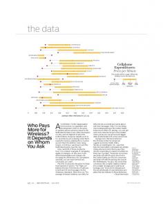
IEEE TRANSACTIONS ON MEDICAL IMAGING, VOL. 18, NO. 5, MAY 1999

385

Resampling of Data Between Arbitrary Grids Using Convolution Interpolation V. Rasche,* R. Proksa, R. Sinkus, P. B¨ornert, and H. Eggers

Abstract—For certain medical applications resampling of data is required. In magnetic resonance tomography (MRT) or computer tomography (CT), e.g., data may be sampled on nonrectilinear grids in the Fourier domain. For the image reconstruction a convolution-interpolation algorithm, often called gridding, can be applied for resampling of the data onto a rectilinear grid. Resampling of data from a rectilinear onto a nonrectilinear grid are needed, e.g., if projections of a given rectilinear data set are to be obtained. In this paper we introduce the application of the convolution interpolation for resampling of data from one arbitrary grid onto another. The basic algorithm can be split into two steps. First, the data are resampled from the arbitrary input grid onto a rectilinear grid and second, the rectilinear data is resampled onto the arbitrary output grid. Furthermore, we like to introduce a new technique to derive the sampling density function needed for the first step of our algorithm. For fast, sampling-patternindependent determination of the sampling density function the Voronoi diagram of the sample distribution is calculated. The volume of the Voronoi cell around each sample is used as a measure for the sampling density. It is shown that the introduced resampling technique allows fast resampling of data between arbitrary grids. Furthermore, it is shown that the suggested approach to derive the sampling density function is suitable even for arbitrary sampling patterns. Examples are given in which the proposed technique has been applied for the reconstruction of data acquired along spiral, radial, and arbitrary trajectories and for the fast calculation of projections of a given rectilinearly sampled image. Index Terms—Arbitrary grids, convolution interpolation, density function, Voronoi diagram.

I. INTRODUCTION

R

ESAMPLING of data between arbitrary sampling grids is important in several medical applications. On the one hand, resampling of data sampled on nonrectilinear grids onto rectilinear grids in the Fourier domain is required for reconstruction of several tomographic techniques such as computer tomography (CT) or magnetic resonance tomography (MRT). On the other hand, resampling of data from rectilinear grids onto nonrectilinear grids becomes important for applications such as the fast calculation of projections.

Manuscript received February 23, 1998; revised April 3, 1999. The Associate Editor responsible for coordinating the review of this paper and recommending its publication was D. Hawkes. Asterisk indicates corresponding author. *V. Rasche, R. Proksa, R. Sinkus, P. B¨ornert, and H. Eggers are with Philips Research Laboratories, Division Technical Systems, Roentgenstrasse 24-26, D-22335 Hamburg, Germany (e-mail: [email protected]). Publisher Item Identifier S 0278-0062(99)05467-1.

Several algorithms for performing reconstructions from data sampled along a nonrectilinear grid have been introduced. Clark et al. introduced a technique treating a nonuniform sample sequence as resulting from a coordinate transformation of a uniform sample sequence [1]. They could show that under certain conditions band-limited functions can be exactly reconstructed from arbitrarily distributed samples. In 1985 O’Sullivan [2] introduced a convolution-interpolation technique based on the original work of Brouw [3] for the reconstruction of CT data. He suggested not to perform a direct reconstruction of the CT data, but to perform a convolution interpolation in the frequency domain from the CT data sampled on a polar pattern onto a rectilinear grid. The final image in the spatial domain was obtained by successively applying a two-dimensional (2-D) Fourier transform. The main advantages of the reconstruction technique introduced inis its reduced computational complexity of in the case of filtered backprojection and stead of its applicability to the reconstruction of data sampled along arbitrary trajectories through the frequency domain. During discretization of the convolution-interpolation technique, the at spatial extent of each sample or the sampling density each sample must be known for correct approximation of the integral. In the case of projection reconstruction tomography or is known analytically and the application of spiral MRT the convolution interpolation is straightforward. Unfortunately, assume ideal trajectories. the analytical expressions for Especially in MRT, this requirement is often not fulfilled. The trajectories may be significantly distorted by nonideal gradient performance [4] causing more or less arbitrary trajectories. Furthermore, gradient waveforms not analytically given can be applied to make full use of the available gradient performance [5], [6]. In some of these cases, however, the corresponding density functions are not available analytically. Although in special cases the density function can be calculated [7], [8], there is a need for algorithms that allow the extraction of the density function from the trajectory itself and several recent publications addressed this problems for spiral-like trajectories in MRT [5], [9]–[11]. A nice overview and comparison between the different techniques is given in [12]. We wish to introduce a different approach using the Voronoi-diagram [13], [14] of the sampling distribution for the determination of the density function. For the 2-D case we define the spatial extent of each pixel according to the area of its Voronoi cell. The calculation of projections as needed for 2-D/3-D registration [15], [16], or for reconstruction techniques such as the algebraic reconstruction technique (ART) [17] or Bayes’ un-

0278–0062/99$10.00  1999 IEEE

386

IEEE TRANSACTIONS ON MEDICAL IMAGING, VOL. 18, NO. 5, MAY 1999

folding [18] is currently done by use of ray-tracing techniques [19]. The computational complexity of projection calculation to can be reduced from an expected performance of if the calculation is applied in the frequency domain, as shown by Napel et al. [20]. Interpolation in the frequency domain, however, causes an intensity modulation in the spatial domain, depending on the interpolation function used. In contrast to Napel et al. we apply a convolution interpolation in the frequency domain using a convolution function, the Fourier transform of which does not have zero values within the desired region of interest in the spatial domain. This allows the pre compensation of the convolution effects in the spatial domain prior to performing the convolution interpolation in the frequency domain. Since the compensation of the convolution-interpolation effects is applied as a pre processing step, the interpolated data in the frequency domain are error free if numerical errors are neglected. This allows interpolation of the Fourier transform of the object function onto an arbitrary grid in the frequency domain. For example, this resampling approach is used for calculation of projections by resampling of the data onto a polar grid in the frequency domain. This new technique has shown promising results in the reconstruction of spiral data sets using an ART-like reconstruction technique [21]. II. THEORY Let and be a Fourier transform pair. The effect of sampling in the frequency domain can be interpreted as with a the multiplication of the continuous function , yielding the sampled data set sampling function

For CT sampling of the data is performed along radial lines yielding a 2–D sampling function as

(4) being the angular increment between sucwith cessive views. The resulting PSF’s have been discussed in the literature [22]–[25] and are not within the scope of this paper. B. Step I: Convolution Interpolation from Arbitrary Grid 1 onto a Rectilinear Grid Convolution interpolation was introduced by Brouw [3] in 1975 and in 1985 a fast sinc function gridding algorithm was introduced by O’Sullivan [2] as an alternative approach for the reconstruction of CT images. The idea was to pass a convoluover the data sampled on the arbitrary tion kernel , with the output of the convolution calculated at grid . For each the uniform intervals on a rectilinear grid point of this rectilinear grid, the convolution kernel centered at this point is used to extract those surrounding samples that contribute to the value and their corresponding weighting. The is given below. The index 1 refers resulting data set to the first step of the algorithm.

(1) (5) can be easily derived from The effect of the sampling to the Fourier convolution theorem [22] as

The Fourier transform of

yields

psf psf

(2)

being the Fourier-transformed sampling function with psf indicating the Fourier or point spread function (PSF), and transform. For MRT, the typical data acquisition in two dimensions is performed on a standard Cartesian grid, yielding a sampling which is a simple 2-D function function

with domain, view.

(6)

Assuming a suitable Cartesian sampling function allows omission of psf and the resulting image can be written as psf (7) . Equation (7) shows that the Fourier with transform of the resampled data set gives the desired image multiplied by the Fourier transform of the convolution kernel and, hence

(3)

(8)

fov being the required interval in the frequency being the image size, and fov being the field of

ensures a nonzero over Appropriate choice of the image, as required to avoid singularities in (8). Suitable kernels are discussed in more detail in [2], [26], [27].

RASCHE et al.: RESAMPLING OF DATA BETWEEN ARBITRARY GRIDS

387

plane lying in all of the dominances of sites in . Formally

over the remaining

(10)

Fig. 1. Example for convex hull in the case of a projection reconstruction data acquisition. Sampling points are indicated as solid circles, sampling points belonging to the inner convex hull are additionally marked by squares, sampling points belonging to the outer convex hull by stars, and the resulting convex hull is marked by the open circles.

Considering a noncontinuous sampling function discrete case of (5) results as

, the (9)

being the area of the frequency domain that is with , and the index indicating samples on assigned to the rectilinear grid. In case of equidistant sampling is constant and causes a scaling of the final image. In case cannot be sepof nonequidistant sampling, however, arated and it is crucial to compensate for the nonconstant over the frequency domain. Mathematically, density of can be seen as the weighting of the th function resulting from the parameter transformation to an equidistant grid as described in more detail in [25]. , as Inspection of (9) shows that the sampling function , must be known in order well as its weighting function to apply a convolution-interpolation. For arbitrary sampling functions, the weighting function is not known analytically and must somehow be extracted from the sampling function itself. 1) Determination of the Weighting Function: We propose to use the area of the Voronoi cell around each sample as a measure for its spatial extent. The definition of the Voronoi diagram is, according to Aurenhammer, the following [14]. Let denote a set of points (sites) in the plane. For two , the dominance of over is defined distinct sites as the subset of the plane being at least as close to as to . Formally

for , denoting the Euclidean distance function. Clearly, is a closed half plane bounded by the perpendicular bisector of and and will be termed the separator is the portion of the of and . The region of a site

The partition of the plane according to (10) is called the Voronoi diagram. To apply this unity-cell approach, the Voronoi diagram is determined via a Delaunay triangulation [13], [28] and the area of each resulting Voronoi cell is used as a measure for the local density of the sampling function. Any general method for the evaluation of the local sampling density faces problems in the region of the outer sampling points. Since the determination of each Voronoi cell requires the existence of neighboring points, it is necessary to properly extrapolate the distribution of points such that reasonable density values can be derived for the outer points. This, in turn, requires some knowledge about the sampling density near the edges of the probed -space region. Therefore, there is no general correct procedure applicable to any arbitrary distribution of points. However, we propose a method which deals with any given -space trajectory and which yields correct results to the first order in the cases of radial and Cartesian sampling strategies. Initially the so-called outer convex hull of all sampling points is determined where the convex hull of a set of points is the smallest convex set that contains the points. Its enclosed . Then, all points belonging to the area is denoted by outer hull are artificially removed from the data set, and the so-called inner convex hull is determined from the remaining . The value distribution with its enclosed area denoted as (11) is thus the scaling factor by which the outer hull is increased (relative to its center of gravity) to generate a correct extrapolation at the edges of the sampled -space region. This result holds to the first order in (with being the spacing between adjacent sampling points) for radial and Cartesian acquisition schemes (see Fig. 1). Different from the common method of embedding the distribution of sampling points into a fixed bounding box, the proposed method is capable of determining the local sampling density function, even at the edges of the sampling grid.

C. Step 2: Convolution Interpolation from the Rectilinear Grid onto Arbitrary Grid 2 For the convolution-interpolation from the rectilinear grid onto the second arbitrary grid, the intermediate image is divided by being the Fourier transform of a second yielding convolution kernel (12)

388

IEEE TRANSACTIONS ON MEDICAL IMAGING, VOL. 18, NO. 5, MAY 1999

(a)

(b)

(c)

Fig. 2. (a) Image and (b) and (c) intensity profile of the ideal software phantom. (c) Zoomed section of (b), as indicated by the vertical lines in (a).

The Fourier transform

of

yields

(13)

on the arbitrary grid can now be calcuThe data lated by applying another convolution interpolation according to

(14) The noncontinuous version of the above technique can be derived according to (9). It should be mentioned explicitly here that the density function is only needed for the convolutiononto . Since the weighting of interpolation from the frequency domain is even during the second convolutiononto , no compensation must interpolation from . be performed for the assigned area of each sample of III. METHOD For evaluation, the new technique was applied to the reconstruction of synthetic data acquired along projection reconstruction, spiral, and arbitrary trajectories. Furthermore, phantom data were obtained along a spiral trajectory with the , according angular speed given by chosen as , to Vlaardingerbroek [29]. With defines a spiral trajectory that behaves like a constant and like a constant linear angular velocity spiral for . The acquisition of the entire data velocity spiral for set was split up into 20 interleaves, each of which use a data acquisition window of 16.8 ms. During data acquisition the eddy-current-compensation boards of the gradient amplifiers were deadjusted to model a less ideal gradient system and to

ensure a significantly distorted trajectory. The actual trajectory of the acquisition was measured, using an approach similar to that given in [30]. All data were acquired on a Gyroscan ACSNT 15 (Philips Medical Systems) equipped with a PowerTrack 6000 gradient system, providing 23 mT/m with 200- s rise time. The software phantom used in simulations to evaluate the new technique is shown if Fig. 2. It consists of several tubes, each of which have a specific diameter and intensity. Its inner structure permits an easy check of the resulting flatness of homogeneous regions, as well as the sharpness. For evaluation of the final image quality, the resulting images themselves and intensity profiles along the marked horizontal line through the image (c.f. Fig. 2) were used. Please note that the software phantom consisted of objects having sharp edges and hence its Fourier transform did not have a limited support in the frequency domain. Since sampling was restricted to a finite area truncation artifacts would arise, even in case of optimal sampling on a rectilinear grid with reconstruction performed using a 2-D Fourier transform. To avoid these high-frequency image artifacts, a simple Gaussian filter was applied to the data calculated in the frequency domain according to (15) being the maximal extent in the frequency with domain required for reconstruction of an image with resolution , as defined by Nyquist’s theorem, and defines the value of the th object at position . In the spatial domain the applied Gaussian shaped filter has a full-width-half-maximum . value of FWHM The second step of the algorithm was evaluated by comparison of images, reconstructed from projections calculated according to the new Fourier-based approach and the standard ray-tracing-based technique, in which a linear interpolation of the image data was used for projection data generation. During all gridding steps a Kaiser–Bessel window defined as [2] (16)

RASCHE et al.: RESAMPLING OF DATA BETWEEN ARBITRARY GRIDS

389

Fig. 4. Voronoi diagram obtained from the sampling pattern of the measured distorted spiral trajectory. The grid points (dots) are omitted in the central region of the frequency domain. In this plot, only the central region of the frequency domain is shown.

with being the zero-order modified Bessel function of the defining the window width, and chosen as first kind, was used as convolution function. Its representation in the spatial domain results [2] (17) During all reconstructions was chosen as four. In the case of projection calculation was chosen as six, and a two-fold oversampling into the radial direction was applied to avoid backfolding caused by the convolution kernel. The Voronoi diagrams were calculated using the QHULL software package distributed by the Geometry Center, University of Minnesota.1 QHULL generates the Voronoi diagram . A preprocessing with an expected performance of step ensures that each grid point is unique during calculation of the Voronoi diagram. After calculation of the Voronoi diagram, the data on the input grid is weighted according to the cell area around each grid point. In the case of multiple acquisitions at a certain grid point, the cell area was divided by the number of coverages. Entire determination of the density function for 64 K samples currently needs about 25 s on a Sun UltraSparc running at 200 MHz. IV. RESULTS A. Reconstruction of Data Sampled Along Arbitrary Trajectories Results obtained using the new Voronoi technique are 1 http://www.geom.umn.edu.

summarized in Figs. 3–5. Fig. 3 summarizes the results obtained with the simulated data. The resulting Voronoi diagrams are shown in Fig. 3(a), (d), and (g) for (a) the projection reconstruction, (d) a constant angular speed spiral, and (g) for a random trajectory through the frequency domain. The resulting images [c.f. Fig. 3(b), (e), and (h)] and intensity profiles [c.f. Fig. 3(c), (f), and (i)] clearly show the quality of the new approach. For projection reconstruction and spiral data acquisition, no difference between the reference [c.f. Fig. 2, dots in Fig. 3(c), (f), and (i)] and the results are visible. In the case of the random trajectory, a four-fold oversampling was performed to avoid severe violation of Nyquist’s theorem. Although the sampling density significantly varies even between neighboring samples, as is clearly visible in the Voronoi diagram shown in Fig. 3(g), the resulting image quality is almost perfect. Some minor deviations are visible in the intensity profiles, which are probably caused by the unknown point-spread function of the random trajectory. Effects such as image blur or enhanced edges, indicating an improperly estimated sampling density function, are not obvious. A quantitative analysis of the resulting error can only be performed for the projection-reconstruction and the spiral trajectories. For both cases, the density functions are known analytically and the resulting images can be compared to those reconstructed using the analytical density function. Taking the images reconstructed with the analytical density functions as a reference, the maximal deviations in the images reconstructed using the Voronoi approach are less 0.5%, and the average error is less than one part per thousand in both cases. Results reconstructed from the phantom data acquired along a distorted spiral trajectory are given in Fig. 5. The corresponding Voronoi diagram is drawn in Fig. 4. Due to the high-sampling density in the center of the frequency domain, the grid points (dots) are omitted in the central region center. Inspection of the graph clearly shows that the radial symmetry of the spiral, as well as its location in the frequency domain, is disturbed. The data are reconstructed using the Voronoi approach [c.f. Fig. 5(a) and (b)], and the fullJacobian-determinant approach [c.f. Fig. 5(c) and (d)] [12]. In the full-Jacobian-determinant approach an analytical density compensation function, based on the Jacobian determinant for the transformation between Cartesian coordinates and the spiral parameters, is derived. Both images, as well as the corresponding intensity profiles, clearly show that both approaches yield almost the same image quality. The maximal difference between both images results to 1% and the average difference is below one part per thousand.

B. Calculation of Projections Fig. 6 shows the comparison between the ray-tracing [c.f. Fig. 6(a), (c), (e)] and the convolution-interpolation approach [c.f. Fig. 6(b), (d), and (f)] for the calculation of projections of a given object. The difference images [c.f. Fig. 6(c) and (d)] between the images reconstructed from the thus calculated projections [c.f. Fig. 6(a) and (b)] and the input image [c.f. Fig. 2(a)] show that the interpolation in the spatial domain causes unsharpness, whereas interpolation in the frequency

390

IEEE TRANSACTIONS ON MEDICAL IMAGING, VOL. 18, NO. 5, MAY 1999

(a)

(b)

(c)

(d)

(e)

(f)

(g)

(h)

(i)

Fig. 3. Voronoi diagrams of sampling patterns acquired along (a) a projection reconstruction, (d) a spiral, and (g) a random trajectory. Images and corresponding intensity profiles obtained using the area of the Voronoi-cell around each sample as a measure for the local sampling density are given in (b) and (c) for the projection reconstruction, in (e) and (f) for the spiral, and in (h) and (i) for the random trajectory. The dots in (c), (f), and (i) indicate the intensity profile of the reference data.

domain produce a slight intensity modulation. The maximal intensity of the appearing deviations from the reference image is 14% in the case of ray tracing and less than 1% in the convolution-interpolation case. These figures have to be carefully interpreted. The maximum deviations in the case of ray tracing appear at the edges, indicating the slight blur caused by the interpolation. The average error is much less and of the same order as that of the convolution-interpolation case. The corresponding zoomed section of the intensity profiles [c.f. Fig. 6(e) and (f)] confirms that the sharpness in the case of convolution interpolation is superior. The

very small intensity variations in the order of less than 1% are not visible. V. CONCLUSION We have shown that resampling of data between arbitrary grids can be performed by applying a two-step convolutioninterpolation algorithm. During the first step, the data are resampled onto a rectilinear grid using a convolution interpolation. As a second step, another convolution interpolation is performed to finally resample the rectilinear data onto the desired output grid. The intermediate resampling of the data

RASCHE et al.: RESAMPLING OF DATA BETWEEN ARBITRARY GRIDS

391

(a)

(b)

(c)

(d)

Fig. 5. Images reconstructed from the data obtained along the distorted spiral trajectory taking the actual trajectory through the frequency domain into account. In (a) the density compensation function (DCF) was obtained using the Voronoi approach, whereas in (c) the DCF was obtained according to the full-Jacobian determinant approach. The intensity profiles (b) and (d) are taken at the indicated lines.

onto the rectilinear grid allows fast compensation of effects caused by the convolutions. The use of the area of the Voronoi cell around each sample, as a measure of the local sampling density, has been shown to be a very reliable and general technique for the estimation of the sampling density function in the case of an arbitrarily distributed sampling pattern. The determined sampling density has been shown to be convincing for the reconstruction of simulated data acquired along projection reconstruction, spiral, and random trajectories through the frequency domain. The application of the new technique to the reconstruction of phantom data acquired along a distorted spiral trajectory has also been shown to produce almost perfect image quality. The Voronoi-diagram approach has been shown to be a very powerful tool for the calculation of sampling density functions. Compared to competing techniques, such as the full-Jacobian-

determinant approach, the Voronoi-diagram approach has the significant advantage that it only depends on the sampling pattern itself and not on the acquisition order. This allows the application of this technique, even in cases where competing techniques may fail, such as intersecting trajectories [12]. Its application as a general tool for density function determination, however, may be limited due to the high computational complexity of the Voronoi diagrams as compared to competing techniques. The second step of the algorithm allows the resampling of data available on a Cartesian grid onto an arbitrary grid. The example of fast calculation of projections shows the high potential of this approach. Although the expected computational complexity is reduced by one order of magnitude compared to the ray-tracing approach, the resulting image quality is convincing. The use of this technique in applications requiring

392

IEEE TRANSACTIONS ON MEDICAL IMAGING, VOL. 18, NO. 5, MAY 1999

(a)

(b)

(c)

(d)

(e)

(f)

Fig. 6. Images reconstructed from the projections calculated via (a) the ray-tracing approach, (b) the introduced convolution-interpolation approach, and (c) and (d) their difference images to the reference data. The corresponding zoomed intensity profiles extracted according to Fig. 2 are given in (e) for the ray-tracing and in (f) for the convolution-interpolation approach.

projections of a given object will significantly speed up the calculation of the projections without sacrificing image quality. ACKNOWLEDGMENT The authors would like to gratefully acknowledge many fruitful discussions with H. Schomberg. REFERENCES [1] J. J. Clark, M. R. Palmer, and P. D. Lawrence, “A transformation method for the reconstruction of functions from nonuniformly spaced samples,” IEEE Trans. Acoust., Speech, Signal Processing, vol. ASSP-33, no. 4, pp. 1151–1164, 1985. [2] J. O’Sulllivan, “A fast sinc function gridding algorithm for Fourier inversion in computed tomography,” IEEE Trans. Med. Imag., vol. MI-4, no. 4, pp. 200–207, 1985.

[3] W. N. Brouw, “Aperture synthesis,” in Methods in Computational Physics, B. Alder, S. Fernbach, and M. Rotenberg Eds. New York: Academic, 1986, vol. 14, pp. 131–175. [4] A. Takahashi and T. M. Peters, “Measurement of k -space trajectories for rf-pulse design,” in Proc 12th Meeting SMRM, 1993, p. 424. [5] D. M. Spielman and J. M. Pauly, “Spiral imaging on a small-bore system at 4.7 t,” Magn. Reson. Med., vol. 34, pp. 580–585, 1995. [6] K. F. King, T. K. F. Foo, and C. R. Crawford, “Optimized gradient waveforms for spiral imaging,” Magn. Reson. Med., vol. 34, pp. 156–160, 1995. [7] J. R. Liao, J. M. Pauly, and N. J. Pelc, “MR imaging using piecewiselinear spiral trajectories,” in Proc. 4th Meeting ISMRM, 1996, p. 390. [8] J. R. Liao and N. J. Pelc, “Image reconstruction of generalized spiral trajectories,” in Proc. 4th Meeting ISMRM, 1996, p. 359. [9] C. H. Meyer, B. S. Hu, D. G. Nishimura, and A. Mcovski, “Fast spiral coronary artery imaging,” Magn. Reson. Med., vol. 28, pp. 202–213, 1992. [10] D. C. Noll, J. A. Webb, and T. E. Warfel, “Parallel data resampling and Fourier inversion by the scane-line method,” IEEE Trans. Med. Imag., vol. 14, no. 3, pp. 454–463, 1995. [11] P. Irarrazabal and D. G. Nishimura, “Fast three dimensional magnetic resonance imaging,” Magn. Reson. Med., vol. 33, pp. 656–662, 1995. [12] R. D. Hoge, R. K. S. Kwan, and G. B. Pike, “Density compensation functions for spiral MRI,” Magn. Reson. Med., vol. 38, pp. 117–128, 1997. [13] M. G. Voronoi, “Nouvelles applications des parameters continus a la theorie des formes quardratiques,” J. Reine Angew. Math., vol. 134, pp. 198–287, 1908. [14] F. Aurenhammer, “Voronoi diagrams—A survey of a fundamental data structure,” ACM Comput. Surveys, vol. 23, pp. 345–405, 1991. [15] L. Lemieux, R. Jagoe, D. R. Fish, N. D. Kitchen, and D. G. T. Thomas, “A patient-to-computed-tomography image registration method based on digitally reconstructed radiographs,” J. Med. Phys., vol. 9, no. 3, pp. 245–261, 1990. [16] J. Weese, T. M. Buzug, C. Lorenz, and C. Fassnacht, “An approach to 2d/3d registration of a vertebra in ct with its profile in x-ray projections,” in CVRMed-MRCAS’97, Lecture Notes in Computer Science 1205. Berlin, Germany: Springer-Verlag, 1997, pp. 119–128. [17] G. T. Herman, Image Reconstruction from Projections: The Fundamentals of Computerized Tomography Orlando, FL: Academic, 1980. [18] G. D’Agostini, “A multidimensional unfolding method based on Bayes’ theorem,” Nucl. Instrum. Meth. Phys. Res., vol. A 362, pp. 487–498, 1995. [19] M. Levoy, “Efficient ray tracing of volume data,” ACM Trans. Graph., vol. 21, pp. 1749–1760, 1994. [20] S. Napel, S. Dunne, and B. Rutt, “Fast Fourier projection for MR angiography,” Magn. Reson. Med., vol. 19, pp. 393–405, 1991. [21] V. Rasche, T. K¨ohler, and R. Proksa, “Iterative reconstruction of MR data sampled along spiral trajectories using convolution-interpolation without knowledge of the density compensation function,” in Proc. 15th Meeting, ESMRMB, Geneva, Switzerland, 1998, p. 352. [22] R. N. Bracewell, The Fourier Transform and Its Applications, 2nd ed. New York: McGraw-Hill, 1986. [23] R. M. Lewitt, “Reconstruction algorithms: Transform methods,” in Proc. IEEE, vol. 71, pp. 390–408, 1983. [24] A. R. Thompson and R. N. Bracewell, “Interpolation and Fourier transformation of fringe visibilities,” Astronom. J., vol. 79, pp. 11–24, 1973. [25] M. L. Lauzon and B. K. Rutt, “Effects of polar sampling in k -space,” Magn. Reson. Med., vol. 36, pp. 940–949, 1996. [26] J. I. Jackson, C. H. Meyer, D. G. Nishimura, and A. Macovski, “Selection of a convolution function for Fourier inversion using gridding,” IEEE Trans. Med. Imag., vol. MI-10, no. 3, pp. 473–478, 1985. [27] H. Schomberg and J. Timmer, “The gridding method for image reconstruction by Fourier transformation,” IEEE Trans. Med. Imag., vol. 14, no. 3, pp. 596–607, 1995. [28] B. N. Delaunay, “Sur la sphere vide,” Bull. Acad. Sci. USSR VII: Class. Sci. Math., pp. 793–800, 1934. [29] J. A. den Boer and M. T. Vlaardingerbroek, Magnetic Resonance Imaging. Berlin, Germany: Springer-Verlag, 1996. [30] G. F. Mason, T. Harshberger, H. Herington, Y. Zhang, G. Prohost, and D. B. Twieg, “A method to measure arbitrary k -space trajectories in rapid MR imaging,” Magn. Reson. Med., vol. 38, p. 492, 1997.