Keywords: gradient adjacent prediction, histogram, reversible data hiding. 1. ...
information by a malicious user during transmission, data hiding has attracted ...
ISS & MLB︱September 24-26, 2013
Reversible Data Hiding Based on Histogram by Using Gradient Adjacent Prediction Y.-C. Lee, Computer Science and Information Engineering, National University of Kaohsiung, Kaohsiung 811, Taiwan. E-mail:
[email protected] H.-H. Chen, Computer Science and Information Engineering, National University of Kaohsiung, Kaohsiung 811, Taiwan. E-mail:
[email protected] C.-Y. Chen Computer Science and Information Engineering, National University of Kaohsiung, Kaohsiung 811, Taiwan. E-mail:
[email protected]
Abstract In this paper, we use gradient adjacent prediction to present a new data hiding method based on histogram. Our method can increase the amount of hidden data, and keep higher PSNR of stego-image. According to experiment results, our method increases the amount of hidden data by 12.5% on the average as compared with Jang et al.’s method. Keywords: gradient adjacent prediction, histogram, reversible data hiding. 1. Introduction Thanks to the flourish of the computer hardware and the Internet, the advanced technologies and their applications advert more and more rapidly. To avoid the interception of sensitive information by a malicious user during transmission, data hiding has attracted significantly much attention [1-7]. The philosophy of data hiding is to embed the secret data into a cover image and to generate quality stego-image with PSNR higher than 40dB. Since the stego-image with PSNR higher than 40dB is imperceptible to human’s recognition, the malicious user will not be able to recognize whether the stego-image is embedded with the secret data or not. Only the specific user can extract the secret data from the stego-image. Two major concerns of data hiding method are the quality of and the amount of secret data embedded in a stego-image. Reversible data hiding method can be categorized as three classes, which are histogram-based methods, Difference Expansion [9], and VQ-Compressed Domain strategies [10]. The histogram-based methods are widely-adopted due to their efficiency and economic computation complexity. In this paper we propose a method derived from the well-known gradient adjacent prediction (GAP) to improve the accuracy of prediction. According to experiment
ISS 273
ISS & MLB︱September 24-26, 2013
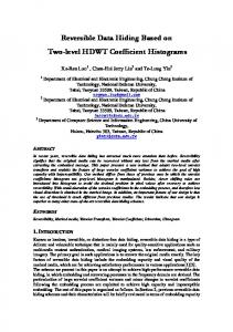
results, our method can increase the amount of hidden secret data, and keep higher PSNR of stego-image. The paper is organized as follows. In Section 2, we review related work. Section 3 presents our method. We give the experiment result in Section 4. The last section concludes this paper. 2. Related Work In this section, we review the algorithm of Jheng et al.’s method [8]. At first, we give the required definitions in this paper. The size of cover image is 512 512 . Pixel (i, j ){0 i, j 511} in the cover image has a pixel value P(i , j ) {P(i , j ) 0 ~ 255 } . The surrounding pixels of pixel (i, j) , Pa , Pb , Pc , Pd , Pe , Pf , Pg , Ph , Pi , Pj , and Pk , are shown as Figure 1. Pa
Pb
Pc
Pd
Pf
Pg
Ph
Pk
Pl
Pm
P( i , j )
Pe
Figure 1. The surrounding pixels of pixel (i, j) Let 4-neighbor set and oblique set of pixel (i, j) be ( i , j ) and (i , j ) , respectively. We then have (i, j ) {(x, y) | x, y [0,511], (i x)2 ( j y)2 1} and (i , j ) {(x, y) | x, y [0,511],(i x) 2 ( j y) 2 2} .
We give the example of (i, j)=(1,1) and get (1,1) (0,1) , (2,1), (1,0), (1,2) , (1,1) { (0,0), (0,2), (2,0), (2,2) } .
The prediction of gradient around pixel (i, j), S(i,j) , is computed by S(i, j ) (D(hi, j ) D(vi, j ) ) (D(li, j ) D(ri, j ) ) , where D(hi , j ) Pl Pm Pg Ph Ph Pk , D(vi , j ) Pg Pm Pc Ph Pd Pk , D(li , j ) Pf Pm Pa Pg Pb Ph , and D(ri, j ) Pd Ph Ph Pm Pe Pk .
We use S ( i , j ) to compute D(i , j ) according to the gradient status as shown in Table 1, which is based on the previous work [8]. In Table 1, (i , j ) and (i , j ) are the total numbers of elements in a
ISS 274
ISS & MLB︱September 24-26, 2013
set of (i , j ) and ( i , j ) , respectively. We further compute D(i , j ) P(i , j ) D(i , j ) .
The previously calculated prediction error are shifted to obtain new prediction error D(i , j ) .
Table 1. The weights of Gradient types S(i , j )
Gradient Type
D( i , j )
Strong Diagonal Similarity
(80, ∞]
(
Diagnol Similarity
(32, 80]
(
Weak Diagonal Similarity
(8, 32]
(
Uniform Similarity
[8, -8]
(
Weak 4-Neighbor Similarity
(-8, -32]
(
4-Neighbor Similarity
(-32, -80]
(
Strong 4-Neighbor Similarity
(-80, -∞]
(
(i , j ) (i , j )
(i , j ) (i , j )
(i , j ) (i , j )
(i , j ) (i , j )
(i , j ) (i , j )
(i , j ) (i , j )
(i , j ) (i , j )
0.2 0.3 0.4 0.5 0.6
0.7 0.8
(i , j ) (i , j )
(i , j ) (i , j )
(i , j ) (i , j )
(i , j ) (i , j )
(i , j ) (i , j )
(i , j ) (i , j )
(i , j ) (i , j )
0.8) 0.7) 0.6) 0.5) 0.4)
0.3) 0.2)
Let M be the secret data to be embedded and Mn be n-th bit of M. We further assume that the sum of peaks of histogram are higher than the length of secret data M. The prediction error D'(i,j) of pixel (i, j) is determined as follows. First we look up Table 1 according to S(i,j), to calculate the prediction of gray value D(i,j). The difference between the predicted value and the actual value of pixel (i, j) is then calculated, and the result is assigned to D'(i,j). Once the histogram of prediction errors is accumulated, two highest peaks are selected and denoted as H1x and H2x. The peaks with zero accumulation closest to these two peaks are then selected and denoted as Z1x, and Z2x. Afterwards, the secret data are embedded using the obtained results. We use Figure 2 to show how to compute D(i , j ) 106 108 98 108 107 99
96 98
91 94
110 110 103 100 94 110 108 106 94 103 112 109 107 105 99 Figure 2. Cover image ISS 275
ISS & MLB︱September 24-26, 2013
According to the pixel value, P(i,j)=103, we calculate D(hi, j ) =9, D(vi, j ) =6, D(li, j ) =12, D(ri, j ) =21 and S( i , j ) =-18. According to S(i,j)=-18, we can figure out that specified pixel is classified to Weak 4-Neighbor. We then compute D(i , j ) ( (i , j ) 0.6 (i , j ) 0.4) =0. (i , j ) (i , j )
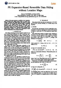
3. Our Method In this section we propose our method. We use a 512 x 512 image to illustrate our method. In order to get more accurate prediction value, we greatly enhance the pixel position of the surrounding pixels from Pa to Pz in Figure 3, instead of Figure 1.
Pa
Pb
Pc
Pd
Pe
Pf
Pg
Ph
Pk
Pl
Pm
Pn
P( i , j ) Po
Pp
Pq
Pr
Ps
Pt
Pu
Pv
Pw
Px
Py
Pz
Figure 3. The new surrounding pixels of pixel (i, j) Thus, the new prediction of gradient around pixel (i, j) is computed by S(i, j ) (D(hi, j ) D(vi, j ) ) (D(li , j ) D(ri , j ) ) , where D(hi , j ) ( Pg Ph Ph Pk Pr Ps Ps Pt ) / 4 , D(vi , j ) ( Pg Pn Pn Pr Pk Po Po Pt ) / 4 ,
D(li , j ) ( Pb Ph Ph Po Po Pu Pf Pn Pn Ps Ps Py ) / 6 , and D(ri , j ) ( Pd Ph Ph Pn Pn Pq Pl Po Po Ps Ps Pw ) / 6 .
Here, D(hi, j ) , D(vi, j ) , D(li, j ) , and D(ri, j ) represent horizontal gradient prediction, vertical gradient prediction, tilted left gradient prediction, and tilted right gradient prediction, respectively. Since the prediction direction and the number of surrounding pixels are different, we introduce the average concept to reduce prediction errors. Let (i , j ) and (i , j ) be the cross and diagonal sets of pixel (i, j) such that (i, j ) {(x, y) | x, y [0,511], (i x)2 ( j y)2 1} and (i, j ) {(x, y) | x, y [0,511],(i x) 2 ( j y) 2 2}.
ISS 276
ISS & MLB︱September 24-26, 2013
We use
S (i , j )
to compute
D(i , j )
according to the gradient status as shown in Table 2. Note that
Table 2 shows the experimental weights of gradient types which are adapted to new surrounding pixels in Figure 3. Table 2. New weights of Gradient types Gradient S(i , j ) D( i , j ) Type Strong (i , j ) (i , j ) ( 1.6 0.8) Diagonal (12, ∞] (i , j ) (i , j ) Similarity (i , j ) (i , j ) Diagonal ( 1.8 0.8) (8, 12] (i , j ) (i , j ) Similarity Weak (i , j ) (i , j ) ( 1.5 0.5) Diagonal (4, 8] (i , j ) (i , j ) Similarity (i , j ) (i , j ) Uniform ( 1.3 0.3) [4, -4] (i , j ) (i , j ) Similarity Weak (i , j ) (i , j ) ( 1.7 0.7) 4-Neighbor (-4, -8] (i , j ) (i , j ) Similarity 4-Neighbor Similarity
(-8, -12]
Strong 4-Neighbor Similarity
(-12, -∞]
(
(
(i , j )
(i , j )
(i , j ) (i , j )
1.8
1.9
(i , j )
(i , j )
(i , j ) (i , j )
0.8)
0.9)
Furthermore, we can calculate the prediction errors as D(i , j ) P( i , j ) D( i , j ) .
(2-1).
To hide the secret data, we generate the space near the peaks by shifting the prediction error D(i , j ) 1 , if Z1x D(i , j ) H1x D(i , j ) D(i , j ) 1 , if H 2 x D(i , j ) Z2x
.
(2-2)
If D(i , j ) is equal to the peaks, it denote that we can embed the secret data Mn .. D(i , j )
D(i , j ) , if D(i , j ) H11 or H12 and if M n 0 . D(i , j ) 1, if D(i , j ) H 11 and if M n 1 D(i , j ) 1, if D(i , j ) H 12 and if M n 1
(2-3)
We can get two pairs of zero and peak points ( H 1x , Z1x ) and ( H 2x , Z 2x ), where Z1x