Hindawi Mathematical Problems in Engineering Volume 2018, Article ID 8014019, 19 pages https://doi.org/10.1155/2018/8014019
Research Article Robust Optimal Navigation Using Nonlinear Model Predictive Control Method Combined with Recurrent Fuzzy Neural Network Qidan Zhu, Yu Han
, Chengtao Cai, and Yao Xiao
College of Automation, Harbin Engineering University, Harbin 150001, China Correspondence should be addressed to Yu Han;
[email protected] Received 5 February 2018; Revised 5 June 2018; Accepted 18 July 2018; Published 13 August 2018 Academic Editor: Julien Bruchon Copyright © 2018 Qidan Zhu et al. This is an open access article distributed under the Creative Commons Attribution License, which permits unrestricted use, distribution, and reproduction in any medium, provided the original work is properly cited. This paper presents a novel navigation strategy of robot to achieve reaching target and obstacle avoidance in unknown dynamic environment. Considering possible generation of uncertainty, disturbances brought to system are separated into two parts, i.e., bounded part and unbounded part. A dual-layer closed-loop control system is then designed to deal with two kinds of disturbances, respectively. In order to realize global optimization of navigation, recurrent fuzzy neural network is used to predict optimal motion of robot for its ability of processing nonlinearity and learning. Extended Kalman filter method is used to train RFNN online. Moving horizon technique is used for RFNN motion planner to guarantee optimization in dynamic environment. Then, model predictive control is designed against bounded disturbances to drive robot to track predicted trajectories and limit robot’s position in a tube with good robustness. A novel iterative online learning method is also proposed to estimate intrinsic error of system using online data that makes system adaptive. Feasibility and stability of proposed method are analyzed. By examining our navigation method on mobile robot, effectiveness is proved in both simulation and hardware experiments. Robustness and optimization of proposed navigation method can be guaranteed in dynamic environment.
1. Introduction During past decades, navigation which can fully reflect artificial intelligence and automatic ability of robot has been an attractive topic [1]. Autonomous navigation is realized in kinds of robots like ground mobile vehicles, unmanned underwater vehicle (UUV), unmanned aircraft, etc. [2–5]. These robots with navigation technology have been applied popularly in various fields such as industry, public service places, transportation, and military [6]. Generally, navigation structure is made up of three main components, perception, decision, and control. Different sensors, such as lidar, inertial measurement unit, GPS, and visual camera, have been used for this purpose generating a series of solutions. This is beyond this paper’s scope. The main problems that this paper prefers to solve are decision and control under assumption of known perception capability. Navigation of robot in objective world is complex for the reasons of existing various uncertainty and nonlinearity
of system [7, 8]. Disturbance or perturbation caused by uncertainty brings challenge to design navigation system. Many inevitable factors lead to uncertainty like dynamic circumstances, sensor noises, and model error [9]. They are coupled and impact together on system. In order to achieve real-time navigation and guarantee safety of robot taking obstacles into account, nonlinear optimal program of robot motion needs to be carried out [10]. However, to make system stable and robust under this condition, control strategy can be tedious and time-consuming. So, effective method should be designed to deal with optimal robust problem of the nonlinear system. Fuzzy logic control is well suited to control robot for its accurate calculation capability and inference capability under uncertainty [11]. Many researchers have implemented this method to deal with navigation of robot. Wang [12] proposed a real-time fuzzy logic control in unknown environment to achieve obstacle avoidance. However, fuzzy logic
2 based method is too sample to deal with complex problem and the structure is less of flexibility. Neural network based approaches have been widely employed in closed-loop control for their strong nonlinear approximation and selflearning capability [13]. Many researches have been done on feedforward multilayer perception neural network for classification, recognition, and function approximation. In [14], recurrent neural network is used to solve optimal navigation problem of multirobot. By constructing formation and using penalty method, navigation becomes convex optimization problem. Recently, fuzzy logic and recurrent neural network structure are combined to form a new structure, i.e., recurrent fuzzy neural network (RFNN). RFNN combines both advantages of neural network and fuzzy logic and earns good nonlinear control capability [15]. In [16], interval type 2 fuzzy neural network is used to control robot. By tuning parameters of structure with genetic algorithm, stable navigation is realized. However, optimization of navigation is not guaranteed and disturbances are not considered in their method. Model predictive control (MPC) has been successfully applied to process industries during past decades for its online optimization programming ability [17]. At each timestep, MPC obtains a finite sequence of control by solving a constrained, discrete-time, optimal control problem over prediction horizon. Current control variable of the sequence is regarded as control law to be applied to the system. By solving the optimal control problem within one sampling interval, MPC can effectively manage MIMO system and hard constraint system. Robust nonlinear MPC (RNMPC) is an active area of research and can easily handle constraint satisfaction against dynamic uncertainty [18]. If a controlled system is ISS with respect to bounded uncertainties, it has a stability margin and is therefore stable with respect to unmodeled dynamics [19]. Many researches have been published using MPC method realizing optimal navigation [20]. In [21], a dual-layer architecture is proposed using MPC and maximum likelihood estimation method to deal with navigation in uncertainty environment. In contrast to our method, it is a kind of probabilistic framework based method. In [22], MPC is also developed to micro air vehicle system generating real-time optimal trajectory in unknown and low-sunlight environments. In [23], autopilot controlling the nonlinear yaw dynamics of an unmanned surface vehicle is designed using MPC combined with multilayer neural network. Inspired by methods mentioned above, a dual-layer control system is designed in this paper. Considering nonlinear nonconvex property of navigation in dynamic environment, RFNN based planner is used to program optimal trajectory of robot. Many methods can be used to train RFNN like backpropagation (BP), genetic algorithm, evolutionary strategy, and particle swarm optimization [24]. Extended Kalman filter (EKF) has attracted many researchers for its characteristics of fast convergence, little limitation in training data, and good accuracy in mathematics process [25]. So, in this paper EKF is used to train RFNN to achieve optimal navigation. A kind of nonlinear robust MPC is then designed to generate actual control command of robot to drive robot to track predictions.
Mathematical Problems in Engineering Considering that there exists intrinsic error between known model and actual model of navigation system of robot, online estimation method needs to be designed. Learning based controller is more adaptive in practical application [26]. By using online data, accurate approximation of the true system model can be constructed. These learning methods mainly consist of Gaussian process and iterative learning methods [27]. In this paper, a specific application based iterative learning method is designed to update system model. The rest of the paper is structured as follows. Section 2 introduces description of problem settled in this paper. Section 3 describes the working of proposed navigation strategy. Section 4 proves stability and feasibility of proposed method. Section 5 illustrates experiments and results and finally Section 6 concludes the proposed scheme.
2. Problem Description In this paper, navigation of robot is realized in unknown environment and the system is nonlinear with constraints. Robust and optimal navigation should be achieved considering dynamic environment and disturbances. Consider the following discrete nonlinear model of robot system: x𝑘+1 = f (x𝑘 , u𝑘 ) + w𝑘1 y𝑘 = h (x𝑘 , u𝑘 ) + w𝑘2 ,
(1)
where u𝑘 ∈ R𝑛1 is control input and x𝑘 , x𝑘+1 ∈ R𝑛2 are system states at time 𝑘 and 𝑘 + 1, respectively. y𝑘 ∈ R𝑛3 is measured output at time 𝑘 and w𝑘1 ∈ R𝑛2 , w𝑘2 ∈ R𝑛3 are process and measurement disturbances, respectively. f(∙) and h(∙) are nonlinear functions where f(∙) is model of system and h(∙) is model of observation. Realistic physical plants are strictly proper, so output function h(x𝑘 , u𝑘 ) can be simplified as h(x𝑘 ). In (1), w1 is model error caused disturbance while w2 mainly contains sensor noise and dynamic environment caused disturbance. Among these uncertainties, dynamic environment changes in random leading to unboundedness of disturbance. On the other hand, model error and sensor noise are bounded and normally are Gaussian that can be estimated. To design useful control method decomposition and combination are used for disturbances as w2 = w2 + w2 .
(2)
Feedback controller is usually designed using y to generate control input u, so (1) changes as x𝑘+1 = f (x𝑘 , u𝑘 ) + w𝑘1 + w𝑘2 y𝑘 = h (x𝑘 ) + w𝑘2 ,
(3)
where w = f(C(w )). C(∙) represents controller. Then, disturbances are separated into two parts, bounded disturbance represented as Δ1𝑘 = w𝑘1 + w𝑘2 and unbounded disturbance represented as Δ2𝑘 = w𝑘2 .
Mathematical Problems in Engineering
3 3.1. RFNN Based Nonlinear Program. Objective function and constraints should be set to realize motion program of navigation. Considering (3), nominal state-space function of robot is represented as
f
x
y
u x
u
z𝑘+1 = f (z𝑘 , k𝑘 ) + 𝐶
w
x
where Δ1 discussed later keeps invariant in this department and is represented as 𝐶 . Objective function reflecting shortest distance can be used:
h
y
C1
(4)
y𝑘 = h (z𝑘 ) ,
C2
Figure 1: Control system considering disturbances.
To achieve navigation, suitable controller should be designed. Considering disturbances divided into two items, we separate strategy into two phases. Real-time program of optimal trajectory is designed at first and robust control of robot is then designed to track the optimal trajectory. In program phase, recurrent fuzzy neural network with moving horizon is designed to plan optimal motion to get robust performance considering Δ2 and can be illustrated as 𝐶1 . After Δ2 is limited, robust model predictive control method is designed in tracking period to deal with Δ1 and can be illustrated as 𝐶2 . Δ1 is decoupled from Δ2 , so Δ2 is not considered during tracking. Then, a controller with dual-layer structure is formed to deal with two kinds of disturbances, respectively. Structure is shown in Figure 1. By separating controller into two parts, bounded and unbounded disturbances are suitably dealt with so that optimal robust performance is realized. Further introduction of control system is in next section.
min
(5)
𝑘
where 𝑑(∙) is distance operator. RFNN structure used here contains five layers and is shown in Figure 3. In order to achieve obstacle avoidance and reach target, output of system is chosen as input of RFNN, i.e., s = y ∈ R𝑛3 , while k = s ∈ R𝑛1 is generated control command to local plant. Subscript 𝑘 is omitted here for simplification. Each node in membership layer performs a membership function. Membership functions can be defined with Gaussian MF as 2
(𝑠𝑖1 − 𝑐𝑖1 𝑗1 )
], (6) = exp [− 𝜎𝑖21 𝑗1 [ ] where exp[∙] is exponential function. c, 𝜎 are the mean and standard deviation of Gaussian function, respectively. The values of them are initially set via expert experience before the strategy begins. As shown in Figure 3, each input parameter has two membership values, so there are 2𝑛3 fuzzy rules in fuzzy rule layer. The firing strength of each rule at current step is determined by outputs of membership layer through an AND operator. The result of each rule is calculated as 𝑠1𝑖1 𝑗1
𝑠2𝑖2 = ∏ 𝑠1𝑖1 𝑗1 .
(7)
𝑗1
3. Control System Design To realize robust optimal navigation of robot, rational framework of control system is designed in this section. Robust nonlinear model predictive controller and recurrent fuzzy neural network based planner are combined to make up the whole control system. Flow diagram is shown in Figure 3 which is extension of Figure 2. Figure 3 emphasizes each part’s function in navigation strategy and is consistent with Figure 2 which mainly explains relationship of uncertainty, controller, and nominal system. The system is made up of nonlinear planner, robust tracker, and local plant. As mentioned in Section 2, there exist kinds of uncertainty bringing disturbances to robot. In order to improve the performance of robot avoiding obstacles and reaching the target, feedback loops that can be used to construct constraints of system are added. Extended Kalman filter is used to train RFNN online to program optimal motion of plant. Iterative online leaning method is used to make system adaptive to disturbance improving performance of MPC.
𝐽 = ∑𝑑 (z𝑘 ) ,
Moreover, a local internal feedback with real-time delay is added to each node of this layer to improve the robustness of the control system. The mathematical form is described by 𝑠3𝑖2 (𝑘) = (1 − 𝛾) 𝑠2𝑖2 + 𝛾𝑠3𝑖2 (𝑘 − 1) ,
(8)
where 𝛾 represents the weight of self-feedback loop and is a constant; s3 (𝑘) is current output of this layer while s3 (𝑘 − 1) represents the last step output. Then, according to the definition of Takagi-Sugeno-Kang (TSK) fuzzy rules, the functions are combined linearly in consequent layer. TSK weight is defined as 𝑛
𝑤𝑖3 𝑖4 = 𝑎𝑖13 𝑖4 𝑧1 + 𝑎𝑖23 𝑖4 𝑧2 + ⋅ ⋅ ⋅ + 𝑎𝑖33𝑖4 𝑧𝑛3 , 𝑛3
(9)
𝑛3
where w ∈ R2 ×𝑛1 , a1 , . . . , a𝑛3 ∈ R2 ×𝑛1 . For the purpose of simplifying calculation, it is assumed that a = a1 = ⋅ ⋅ ⋅ = a𝑛 . The output of this layer can be computed as follows: 𝑠4𝑖4 = ∑𝑤𝑖3 𝑖4 𝑠3𝑖2 . 𝑖3
(10)
4
Mathematical Problems in Engineering
Control system
x0 , xd ,
Nonlinear planner
Robust tracker
z, v
u
EKF
y
Robot
NMPC
RFNN
Local plant
Localizer
IL
Figure 2: Block diagram of control system.
PM NM PM NM
s
s
is constant covariance matrix of measurement error. Q𝐸𝐾𝐹 𝑘 matrix and is set according to [28], P is covariance matrix of estimation error, and I is identity matrix. O is orderly derivative matrix of observation vector with respect to RFNN weights. Constraints of obstacles and target during navigation process are achieved by establishing observation vector in (13); Jacobian matrix is then calculated to predict weights of RFNN: O=
PM NM
Figure 3: Structure of RFNN.
Activation function is set at each node of output layer to limit output forming output constraint: 𝑠𝑖4
=
𝑠4𝑖4
, 1 + 𝜂𝑖4 𝑠4𝑖4
(16)
Target constraint is always prior. Only when obstacles threaten safety of robot, is obstacle constraint considered in (13). As initial weights are generated in random, by repeating calculation suboptimal trajectory can be got satisfying (4). Calculation time is t depending on repetition. To deal with uncertainty caused by dynamic environment, moving horizon is used forming online dynamic program. 𝑇𝑟𝑎1 , . . . , 𝑇𝑟𝑎𝑛 are trajectories generated in different horizon. 𝑡Δ is time between contiguous horizons. Time constraint should be satisfied: 𝑡 < 𝑡Δ ,
(11)
where 𝜂 is constant and its value depends on practical application. In order to achieve motion program, extended Kalman filter method proposed in [28] is modified to train the weights of RFNN structure online. At step k, the EKF function is expressed as follows:
𝜕o𝑇 . 𝜕a
(17)
where 𝑡Δ depends on uncertainty. A new variable is set to judge disturbance using quadratic form as 𝑝
𝑇
𝑝
Δ = (o𝑘 − o𝑟𝑘 ) QΔ (o𝑘 − o𝑟𝑘 ) ,
(18)
𝑝
where o𝑘 and o𝑟𝑘 are observation vectors at each step of program trajectory under system (4) and real trajectory under system (3), respectively. QΔ is matrix of weights. Upper bound is set to get
a𝑘+1 = a𝑘 − K𝐸𝐾𝐹 e𝐸𝐾𝐹 , 𝑘 𝑘
(12)
e𝐸𝐾𝐹 = o𝑘 − o𝑑𝑘 , 𝑘
(13)
Δ < Δ 𝑏𝑜𝑢𝑛𝑑 ,
(14)
According to (4)∼(19), global motion program is obtained with bounded Δ2 . However, during practical process there exists Δ1 affecting performance of navigation. So, suitable control and online learning method are needed in tracking procedure to guarantee robustness of system and ensure effective estimation of disturbances.
K𝐸𝐾𝐹 𝑘
=
P𝑘 O𝑘 [R𝐸𝐾𝐹 𝑘
+
−1 O𝑇𝑘P𝑘 O𝑘 ]
+ [I − K𝐸𝐾𝐹 O𝑇𝑘] P𝑘 , P𝑘+1 = Q𝐸𝐾𝐹 𝑘 𝑘
,
(15)
where K𝐸𝐾𝐹 is Kalman gain matrix. e𝐸𝐾𝐹 is estimation error. o𝑑 is desired value of o which is observation vector. R𝐸𝐾𝐹 is
(19)
Mathematical Problems in Engineering
5
3.2. Learning Based Robust Tracking
2
3.2.1. Robust Nonlinear Model Predictive Control. Tube-based robust nonlinear model predictive control makes closed-loop trajectory, in the presence of disturbances, lie in a tube whose center is nominal trajectory. In this paper, nominal trajectory is generated by RFNN motion planner and then a tubebased approach is adopted to tracking system considering uncertainty caused by model and location error. Considering (3) and (4), robot system to be controlled is the following nonlinear state-space form with bounded disturbances and Δ2𝑘 is not included: x𝑘+1 = f (x𝑘 , u𝑘 ) + Δ1𝑘 ,
(21)
𝑇
𝑇
+ (u − k𝑙 ) R (u − k𝑙 ) + 𝐽𝑓 (x; z𝑓 , 𝑙) ,
(22)
where Q ∈ R𝑛2 ×𝑛2 and R ∈ R𝑛1 ×𝑛1 are positive definite. z𝑙 ∈ Z and k𝑙 ∈ V are reference trajectory and control action, respectively. 𝐽𝑓 (∙) is terminal cost function and z𝑓 is terminal state that is changing due to (21). Optimal control problem can be illustrated as min 𝑢
𝐽 (x, u, 𝑘, 𝑙) .
(23)
The solution of (23) is u∗ = {u∗0 , u∗1 , . . . , u∗𝑁−1 } and associated ∗ state trajectory is x∗ = {x0∗ , x1∗ , ..., x𝑁−1 }. 𝜅 = u∗0 is applied to uncertainty system, i.e., the first element in the sequence. If x = z𝑙 , then u = k𝑙 , so that 𝐽(x, u, 𝑘, 𝑙) = 0. Minimum value of cost function at each step of trajectory is represented as 𝐽min (x, 𝑘, 𝑙). Level set of cost function defines a neighborhood of nominal trajectory. A tube can be defined [29]: 𝑆𝑑 = {x | 𝐽min (x, 𝑘, 𝑙) ≤ 𝑑} .
start
k
End
Figure 4: Dynamic iterative route.
According to [30], stable condition exists:
representing trajectories and update interval in different horizon. Only the first 𝑡Δ step of 𝑇𝑟𝑎 is valid motion. And interpolation is applied to get tightened Z and V. Considering deviation of state and control between actual system and nominal system, cost function to be minimized is defined as 𝐽 (x, u, 𝑘, 𝑙) = (x − z𝑙 ) Q (x − z𝑙 )
k
(20)
where f(∙) is twice continuously differentiable. If cost function of MPC is Lipschitz continuous; there exist two invariant sublevel sets of X such that the smaller set is robustly asymptotically stable for controlled system with a region for attracting the larger set [29]. Planned state and control input of navigation system in Section 3.1 are chosen as nominal state and control represented as Z, V respectively. The controller aims at steering robot with disturbances close to index prediction and keeping actual trajectory of robot in a tube with good robustness. However, nominal state and control provided above are finite and the whole trajectory keeps changing as introduced in (17) ∼ (19). To obtain effective and tightened reference sets, the following procedure is used. An object is defined as T = {(𝑇𝑟𝑎1 , 𝑡Δ1 ) , (𝑇𝑟𝑎2 , 𝑡Δ2 ) , . . . , (𝑇𝑟𝑎𝑙 , 𝑡Δ𝑙 ) , . . .} ,
1
(24)
𝑇
min {𝐽 𝑓 (f (x,u) ; z𝑓 , 𝑙) + (x − z𝑓 ) Q (x − z𝑓 ) u 𝑇
(25)
+ (u − k𝑓 ) R (u − k𝑓 )} ≤ 𝐽 𝑓 (f (x, u) ; z𝑓 , 𝑙) , where 𝐽 𝑓 (f(x, u); z𝑓 , 𝑙) = (f(x, u) − z𝑓 )𝑇Q𝑓 (f(x, u) − z𝑓 ) and x ∈ {x | 𝐽 𝑓 (x; z𝑓 , 𝑙) ≤ 𝛼}. Q𝑓 is positive definite. Then 𝐽𝑓 (∙) is determined as 𝐽𝑓 (x; z𝑓 ) = 𝑑𝐽 𝑓 (x; z𝑓 )/𝛼. Method in [31] is used to solve the optimization problem. 3.2.2. Iterative Online Learning. In actual situation there are disturbances caused by inaccurate model established a priori and invariant perception error. So, online learning method should be considered to estimate intrinsic part of disturbances online and make the control system effective. As f(∙) is nonlinear in (20), disturbance Δ1 is no more Gaussian leading to the fact that GP based estimation method is not suitable here. So, a kind of PD iterative online learning method is designed in this section to estimate disturbances. The process is assumed to occur in an unknown environment and robot moves to goal avoiding obstacles in a predictive routine instead of a known iterative path. So, compared to traditional iterative method dynamic iterative route is used in our iterative learning algorithm. In order to learn compensation with dynamic route, suitable and effective iterative function should be designed as follows. Kinematic model of mobile robot is used here to introduce the procedure and detailed information is introduced in Section 5.1. Then state-space system in (20) can be illustrated as 𝑓 (x, u, w) = x + A (x) u + Δ1 ,
(26)
where x is state of system, u is control input, and Δ1 is disturbance need to be learned. Each iteration has 𝑘 equations, but start and end points are different. The demonstration of choosing iteration route is illustrated intuitively in Figure 4. There are two trials end at points 1 and 2, respectively, during the process; start points can be got due to same steps 𝑘.
6
Mathematical Problems in Engineering
In order to use this form of iterative route, a new variable is defined: 𝜎 = z − x. According to (26), 𝑘 equations can be got: 𝜎2 = z2 − x2 = z2 − x1 − A1 u1 − Δ1 = z1 − x1 + A1 k1 − A1 u1 − Δ1
e𝐾 = 𝜎𝑑 − 𝜎𝐾 ,
= 𝜎1 + A1 k1 − A1 u1 − Δ1 𝜎3 = z3 − x3 = z2 − x2 + A2 k2 − A2 u2 − Δ2
(27)
= 𝜎2 + A2 k2 − A2 u2 − Δ2
(31)
where 𝜎𝑑 represents desired error between actual state and optimal predictive state and it is usually 0. Substituting (31) and (28) into (30) yields closed-loop iteration dynamics: Δ𝐾+1 = (I + (𝜆𝑝 R𝐼𝐿 + 𝜆𝑑 (I − R𝐼𝐿 )) B) Δ𝐾
= 𝜎1 + A1 k1 − A1 u1 + A2 k2 − A2 u2 − Δ1 − Δ2
+ (𝜆𝑝 R𝐼𝐿 + 𝜆𝑑 (I − R𝐼𝐿 )) (𝜎𝑑 − 𝜎0 ) .
.. ., where z, k, and A are variables of references produced by RFNN in Section 3.1. In order to simplify representation, Δ1𝑘 is replaced by Δ𝑘 above. Then the lifted form can be organized as 𝜎𝐾 = 𝜎0 − BΔ𝐾 ,
(28)
where 𝐾 represents iteration and B is lower triangular matrix. Component of each item is shown as [ [ [ 𝜎𝐾 = [ [ [
where 𝜆𝑝 and 𝜆𝑑 are proportional and derivative learning gains, respectively. R𝐼𝐿 is lower triangular Toeplitz matrix derived from column vector [0, I, 0, . . . , 0]𝑇 where 0 is matrix with 0 elements and I is 𝑛2 × 𝑛2 unit matrix. For iteration 𝐾, error can be defined as
𝜎2
𝜎3 ] ] ] , .. ] ] . ]
[𝜎𝑘+1 ] 𝜎1 + A1 k1 − A1 u1 ] [ [𝜎1 + A1 k1 − A1 u1 + A2 k2 − A2 u2 ] ] [ ], 𝜎0 = [ ] [ .. ] [ . ] [ 𝜎1 + ⋅ ⋅ ⋅ + A𝑘 k𝑘 − A𝑘 u𝑘 ] [
(29)
According to [33], iterative learning process is asymptotically stable, if 𝜌 (I + (𝜆𝑝 R𝐼𝐿 + 𝜆𝑑 (I − R𝐼𝐿 )) B) < 1,
4. Stability Analysis According to Figure 2, the control system is made up of two parts. So, in order to analyze stability of the system, each part’s stability should be guaranteed. 4.1. Convergence of Recurrent Fuzzy Neural Network. In this paper, a training method based on EKF is used as shown in Section 3.1. Appropriate parameters should be designed. Then, by iteratively calculating (12) ∼ (15) trajectories are generated. By evaluating these trajectories, suboptimal trajectory is chosen. Observation vector, o𝑘 , is first expanded at final stable weights a𝑑 as 𝜕o + 𝜉𝑘 , 𝜕a
𝐸𝑘 = e𝑇𝑎𝑘 P𝑇𝑘e𝑎𝑘 .
[Δ𝑘 ] Although the system illustrated by (26) is nonlinear, it is Lipschitz continuous. According to [32], linear method can deal with this kind of problem well. Compared to nominal discrete-time system introduced in [33], the initial conditions in (28) are different at each iteration. Many methods can be used to settle this problem such as initial state learning mechanism or smooth interpolation. As shown above, 𝜎0 is made up of discrepancy at all steps in each trajectory. Suppose the first two iterations are convergent, then 𝜎0 decreases in later iteration and is upper bounded. So, a simple forgetting factor 𝜆 𝑓 is used to discount integration effect of iterative learning. Then a kind of PD-type iterative learner is used: Δ𝐾+1 = 𝜆 𝑓 Δ𝐾 + 𝜆𝑝 R e𝐾 + 𝜆𝑑 (I − R ) e𝐾 ,
(34)
where 𝜉𝑘 is first-order approximation residue and O(∙) is mapping function from weights to observation. Error of weights can be defined: e𝑎𝑘 = a𝑘 − a𝑑 . Then, Lyapunov function can be chosen as
[Δ ] [ 2] [ ] Δ𝐾 = [ . ] . [ . ] [ . ]
𝐼𝐿
(33)
where 𝜌(∙) is spectral radius operator.
o𝑘 = O (a𝑑 ) + (a𝑘 − a𝑑 )
Δ1
𝐼𝐿
(32)
(30)
(35)
The difference can be calculated as Δ𝐸 (𝑘) = 𝐸 (𝑘 + 1) − 𝐸 (𝑘) 𝑇 −1 = e𝑇𝑎(𝑘+1) P−1 𝑘+1 e𝑎(𝑘+1) − e𝑎𝑘 P𝑘 e𝑎𝑘
(36)
𝑇
< [e𝑎(𝑘+1) − e𝑎𝑘 ] P−1 𝑘 e𝑎𝑘 −1
− e𝑇𝑎(𝑘+1) [P𝑘+1 − Q𝐸𝐾𝐹 ] P𝑘 O𝐸𝐾𝐹 𝐻−1 𝑘 𝑘 𝑘 𝜉𝑘 , where 𝐻𝑘 = R𝐸𝐾𝐹 + O𝑇𝑘P𝑘 O𝑘 . Then following inequation can 𝑘 be got according to [28] Δ𝐸𝑘
2 3𝑜𝑘 𝜉𝑘 2 2 , 𝑚 (e𝑘 − 3 𝜉𝑘 )
(39)
(40)
with 99.99% 𝜉𝑘 being bounded. And 𝑟(𝑘) adaption law is got: 2 3𝑜 1 e𝑘 𝑟𝑘 = ( + 𝑘), 2 64𝑚 𝑚
(41)
which can make control system’s error convergent, i.e., bounded e𝑘 . As mentioned in Section 3.1, initial weights are generated in random leading to predictive trajectories being different with different initial weights. Initial weights are represented as {a10
a20
⋅⋅⋅
a𝑙0
⋅ ⋅ ⋅} ,
2 𝐽min (x, 𝑘, 𝑙) ≤ 𝐽 (x, u∗ , 𝑘, 𝑙) ≤ 𝑑1 x − z𝑙0 .
(43)
Stability condition is established in (25); then 𝐽min (x, 𝑘 + 1, 𝑙) ≤ 𝐽min (x, 𝑘, 𝑙) 𝑇
− (x − z𝑙0 ) Q (x − z𝑙0 )
(44)
𝑇
− (𝜅𝑘 − k𝑙0 ) R (𝜅𝑘 − k𝑙0 ) . There is also lower bound due to weight matrix Q, so 2 𝐽min (x, 𝑘, 𝑙) ≥ 𝑑2 x − z𝑙0 .
(45)
Combine (43) ∼ (45), and
where each element of 𝜉𝑘 is normal distribution as 𝜉𝑖𝑘 ∼ 𝑁(0, 𝑟𝑘 ); then 2 e 3𝑜𝑘 < 𝑟𝑘 < 𝑘 , 𝑚 64𝑚
For each trajectory in T, suppose there is 𝑑 > 𝑑 and bounded area around trajectory is 𝑆𝑑 = {x | 𝐽min (x, 𝑘, 𝑙) ≤ 𝑑 }. Let x∗ = z denotes generated state of nominal system; i.e., x𝑘+1 = f(x𝑘 , u𝑘 ) + C, with input u∗ = k. Since f(∙) is Lipschitz continuous, ‖x𝑘∗ −z𝑙𝑘 ‖ ≤ 𝐿‖x−z𝑙0 ‖ for all x ∈ 𝑆𝑑 +Δ1 . According to (22) and (25), there exists 𝑑1 such that
(42)
where each element corresponds to an independent trajectory produced by EKF training method. Some method can be chosen to learn initial weights, but a simple method of iteration is used to economize computation cost and guarantee real-time program ability. Considering practical condition, evaluation of optimal trajectory is different especially in dynamic navigation problem. With evaluation criteria, a0 is chosen to obtain suboptimal trajectory.
𝐽min (x, 𝑘 + 1, 𝑙) ≤ (1 −
𝑑2 min ) 𝐽 (x, 𝑘, 𝑙) . 𝑑1
(46)
In practice, the surroundings where robot needs to achieve navigation can be entirely or partially detected by sensors. Suppose the change of surroundings is continuous and not too fast relative to robot’s motion. Then disturbance Δ1 is bounded. Let Δ = max{‖Δ‖ | Δ ∈ Δ1 }. According to [29], for all x ∈ 𝑆𝑑 and x𝑘+1 = f(x𝑘 , u𝑘 ) + Δ1 , there is a constant 𝑑3 such that 𝐽min (x, 𝑘 + 1, 𝑙) ≤ (1 −
𝑑2 min ) 𝐽 (x, 𝑘, 𝑙) + 𝑑3 Δ1 𝑑1
𝑑 ≤ (1 − 2 ) 𝐽min (x, 𝑘, 𝑙) + 𝑑3 Δ. 𝑑1
(47)
If (𝑑2 /𝑑1 )𝐽min (x, 𝑘, 𝑙) ≥ 𝑑3 Δ, (47) becomes 𝐽min (x, 𝑘 + 1, 𝑙) ≤ 𝐽min (x, 𝑘, 𝑙) ≤
𝑐1 𝑐3 Δ . 𝑐2
(48)
So, there exists constant 𝑑 = 𝑐1 𝑐3 Δ/𝑐2 that limits actual path of robot in a tube of optimal trajectory generated by RFNN. After analysis and design of the overall system, whole strategy of navigation is illustrated as Algorithm 1.
5. Experiments 4.2. Stability and Robustness of Nonlinear Model Predictive Control. By using RFNN based planner, a set of trajectories are obtained in (21) to approximate optimal path in dynamic environment. MPC method is then used to limit states of robot in a tube around the optimal path under disturbance Δ1 .
5.1. Model of Mobile Robot. In order to approve effectiveness of our control system, a kind of differentially driven mobile robot system model in [9] is used here. The robot model in unknown environment with obstacles and target is illustrated as in Figure 5.
8
Mathematical Problems in Engineering
Initialization: x0 = 0, obtain initial position of target and obstacles, x𝑡𝑎𝑟𝑔𝑒𝑡 , x𝑜𝑏𝑠𝑡𝑎𝑐𝑙𝑒 . set c, 𝜎, QΔ , 𝛾, 𝜂, Δ 𝑏𝑜𝑢𝑛𝑑 , Q, R, (𝑑/𝛼)Q𝑓 , 𝜆 𝑓 , 𝜆𝑝 , 𝜆𝑑 while ‖x − x𝑡𝑎𝑟𝑔𝑒𝑡 ‖>𝛽 do Prediction: Predict robot motion according to (4) ∼ (16) and (33) ∼ (39). Generate trajectory in T as well as referential states and control commands, i.e. z, k. while Δ < Δ 𝑏𝑜𝑢𝑛𝑑 do Tracking: Generate actual control command, u, according to (21) ∼ (30). Sensor: Measure distance and angel information among target, obstacles and robot, i.e. y. Location: Estimate state of robot, obstacle and target, i.e. x, x𝑡𝑎𝑟𝑔𝑒𝑡 , x𝑜𝑏𝑠𝑡𝑎𝑐𝑙𝑒 . Update Δ, x, x𝑡𝑎𝑟𝑔𝑒𝑡 , x𝑜𝑏𝑠𝑡𝑎𝑐𝑙𝑒 . Algorithm 1: Navigation strategy.
Table 1: Initialization of parameters. O1
O2
𝑏
Target
c dg
Y
w
Obstacle
l
do
𝜎 𝜂 𝛾
0.2m 𝜋 𝜋 0 0 − − [ 2 2] [ 𝜋 ] 𝜋 10 5 2 2 ] [ [2.5 1 1 1] [0.3 0.3 ⋅ ⋅ ⋅] 0.3
Δ 𝑏𝑜𝑢𝑛𝑑
0.5
𝜆𝑝
0.1
𝜆𝑑 𝜆𝑓 𝛽
3 0.9 0.5
g R
o
b
(x, y)
X
r
Figure 5: Model of mobile robot in unknown environment.
Robot is motivated by right and left wheels, [V𝑟 , V𝑙 ]𝑇. Linear and angular velocities are V + V𝑙 , V= 𝑟 2 V − V𝑙 , 𝜔= 𝑟 2𝑏 V + V𝑙 𝑅=𝑏 𝑟 , V𝑟 − V𝑙
(49) (50) (51)
Difference equation is then illustrated as
x𝑘+1
cos 𝜃𝑘 0 [ sin 𝜃 0] = x𝑘 + Δ𝑡 [ ] u𝑘 , 𝑘 [ 0
(52)
1]
where u = (V, 𝜔)𝑇. x𝑘 , x𝑘+1 are robot’s postures at 𝑘 and 𝑘 + 1 steps, respectively, and are represented as x = [𝑥, 𝑦, 𝜃]𝑇. Distance and angle of target and nearest obstacle corresponding to robot are chosen as measurement, so output is represented as 𝑇
y𝑘 = [𝑑𝑔𝑘 , 𝜃𝑔𝑘 , 𝑑𝑜𝑘 , 𝜃𝑜𝑘 ] .
(53)
As shown in Figure 5, a sparse representation of obstacles is used to train RFNN. Circles with center on obstacle represent dangerous area. Radius of circle depends on EKF learning method and estimation error. Location of obstacle is usually not accurate leading to error of centers’ position shown in figure. Distance between 𝑂1 and 𝑂2 depends on 𝑏. Although RFNN structure is convergent, robot will vibrate at terminal position due to feedback control principle. When robot reaches area determined by 𝛽, a brake control is used. 5.2. Performance in Static Condition with Bounded Disturbance. Simulation experiment is carried out using Matlab. Activity space is limited in 10 m × 10 m. There exist obstacles and target. Mobile robot needs to reach target and avoid obstacles. Constant parameters to be initialized are listed in Table 1. The weight matrices are set with 25 : 15 : 1 ratio weighting position-tracking error and linear and angular velocity control input in (22). The weight QΔ is switched between two sets due to position corresponding to target and obstacles. Proposed method is first examined in static environment. As environment is static, only one prediction of optimal motion of robot is generated and the weights of RFNN are shown in Figure 6. There is no drastic variety underlying smoothness of process. Gaussian noise with mean zero and variance of 0.03 is injected to system named as disturbance 1. And 20 trajectories are generated under random disturbance. Performance is shown as in Figure 7. All trajectories are bounded in a band. Each trajectory of robot can realize reaching adjacent area of target and avoiding obstacles. Optimal and robust navigation is achieved. Position error curves of robot are shown in Figure 8(a), which are bounded in a narrow band. Figures 8(b) and 8(c) represent linear
Mathematical Problems in Engineering
9 Changes of weights
60 50
Weight
40 30 20 10 0
0
10
20
30 Time
40
50
60
Figure 6: Weights of RFNN. Disturbance
Disturbance
0.1
Path
8
0.05 0 −0.05 −0.1
Target 0
25 50 Time
Static obstacle
70
6 Path
5 4 4.5 Y (m)
Y (m)
Dynamic obstacle
Robot
2
4 0 Start 0
3.5 2
4 X (m)
6
8
4
4.5
5
5.5
X (m)
Figure 7: Performance in static environment: 20 trajectories with disturbance 1.
and angular velocities of robot, respectively. They are not narrow contrasted to position error for the reason that input commands should control robot against random disturbance and limit robot’s position in a narrow tube. Computation cost of generating optimal control command at each step is shown in Figure 9. Lines in red are average values. 5.3. Performance of Online Iterative Learning Method. In order to examine online iterative learning method proposed,
Gaussian noise with mean 0.1 and variance of 0.03 is injected to system named as disturbance 2. 20 trajectories are also generated under this random disturbance. Performance is shown as Figure 10. For neat expression only one trajectory without iterative learning in magenta is shown in figure. This trajectory is dangerous and does not lie in stable tube. Trajectories with iterative leaning are illustrated in cyan and are same as trajectories under disturbance 1 underlying estimation method which is effect. Estimation of disturbance
10
Mathematical Problems in Engineering Position error 10 Position error 5.2
8
Distance (m)
Distance (m)
5 6
4
4.8 4.6 4.4
2
4.2 30
0 0
10
20
30 40 Time
50
60
31
32 33 Time
34
35
70
(a) Distance error of robot
Linear velocity
0.6
Angular velocity (rad/s)
Linear velocity (m/s)
0.5 0.4 0.3 0.2 0.1 0
Angular velocity
0.2
0
20
40 Time
60
(b) Linear velocity of robot
0.1
0
−0.1
−0.2
0
20
40 Time
60
(c) Angular velocity of robot
Figure 8: Position error and control inputs of robot with 20 trajectories. Computation cost
2
between two conditions. The largest bias at each point of 20 trajectories under two conditions is shown in Figure 12. The largest bias of trajectories under disturbance 2 is a little higher.
Computation cost (s)
1.5
1
0.5
0 0
20
40 Time in samples
60
Figure 9: Computation cost at each step of 20 trajectories.
2 is shown in Figure 11. Detailed information is shown in Table 2. There is not much difference of values in each item
5.4. Comparison with Other Methods. The main novelty of proposed method in this paper is that a motion planning and control method based navigation strategy is proposed to deal with uncertainty and guarantee robust optimization of the process. The dual-layer structure is designed to be feasible and effective by combining RFNN and MPC method. Many motion planning techniques are used to achieve navigation, like potential field method, sampling based planner, interpolation curve method, A∗, neural network, fuzzy logic, genetic algorithm, particle swarm optimization, etc. A∗ method is widely used in autonomous vehicles for its efficiency [34]. Furthermore, OPTI toolbox of Matlab includes many optimal solvers that can be used to design nonlinear planner. In order to introduce our method’s effectiveness, A∗ method together with OPTI based numerical optimization method is compared with ours. As control policy is considered in our method, PID method in [35] is used for two planners
Mathematical Problems in Engineering
11 Disturbance
Disturbance
0.2 0.1 0
Path
8
Target
0
7
25 50 Time
6
Path
5 Dangerous
4 4.5 3 Y (m)
Y (m)
5
70
Robot
2
4 1 0
3.5
Start −1
0
2
4 X (m)
6
4
8
4.5
5
5.5
X (m)
Trajectory with IL Trajectory without IL
Figure 10: Performance in static environment: 20 trajectories with disturbance 1.
Table 2: Evaluation of trajectories in static environment. Prediction cost (s)
Step
Average distance (m)
Average terminal error (m)
Average bias (m)
4.13 4.13
63 63
9.82 9.86
0.36 0.35
0.061 0.067
Trajectories under disturbance 1 Trajectories under disturbance 2
Estimation
0.2
Estimation
0.15
0.1
0.05
0
−0.05
0
25
50 Time
Figure 11: Estimation of disturbance 2.
70
above forming complete navigation system just like ours. Performance is shown in Figure 13. A∗ method just plans positions of robot, leading to bad tracking performance under disturbance which is reflected by tracking error in Table 3 and the path in red with rectangle marks. The trajectory is not smooth contrasted to our method and OPTI and PID method. PID control method that lacks online learning mechanism fails to drive robot to target when disturbance in Figure 10 acted on system, which is reflected by red path with triangle marks. Compared to A∗ and PID based strategy, OPTI and PID method that plans motion performs better. But OPTI based planner takes up too much computation cost reflected in Table 3 leading to bad realtime planning ability. Detailed information of these methods’ performance is illustrated in Table 3. It is proved that our method can achieve good online navigation. 5.5. Performance in Dynamic Condition. Proposed method is then examined in dynamic environment. Performance is
12
Mathematical Problems in Engineering
Table 3: Comparison between our method and others. Distance (m) 10.132 10.389 6.209 10.090
OPTI & PID A∗ & PID 1 A∗ & PID 2 OURS
Step 60 62 37 62
Computation cost (s) 37.891 0.512 0.512 3.142
Bias
0.3
Terminal error (m) 0.289 0.402 3.889 0.251
Tracking error (m) 0.048 0.059 0.231 0.040
Bias
0.4
0.3
Bias (m)
Bias (m)
0.2 0.2
0.1 0.1
0 0
20
40 Time
60
0
(a) Maximal bias under disturbance 1
20
40 Time
(b) Maximal bias under disturbance 2
Figure 12: Largest bias at each step under two conditions.
Path
8
Target Static obstacle 6 Dynamic obstacle Y (m)
0
4
Robot
2
0 Start 0
2
4
6
8
X (m) OPTI+PID A∗+PID1 A∗+PID2 OURS
Figure 13: Comparison between our method and others.
60
Mathematical Problems in Engineering
13 Path
8
Target
Target
7 6 5
6 Dynamic obstacle Y (m)
4
Y (m)
Path
8
3 2
4
2
Robot
1 0 −1
Robot
0
Static obstacle Start 0
2
4 X (m)
6
Start 0
8
2
4 X (m)
Real trajectory Predictive trajectory Target trajectory
Real trajectory Predictive trajectory Target trajectory
(a) 𝑘 = 1
(b) 𝑘 = 10
Path
8
6
8
Path
8 Target
6
6 Y (m)
Y (m)
Robot 4
4
Target
Robot 2
2
0
0 Start 0
2
4 X (m)
6
Start 0
8
Real trajectory Predictive trajectory Target trajectory
6
8
(d) 𝑘 = 55
Path
Path
8 Robot
6
6
4
Y (m)
Y (m)
4 X (m)
Real trajectory Predictive trajectory Target trajectory
(c) 𝑘 = 18
8
2
2
4 Robot 2
Target
Target
0
0 Start 0
2
4 X (m)
6
8
Start 0
Real trajectory Predictive trajectory Target trajectory
2
4 X (m)
Real trajectory Predictive trajectory Target trajectory
(e) 𝑘 = 97
(f) 𝑘 = 126
Figure 14: Continued.
6
8
14
Mathematical Problems in Engineering Path
8
Y (m)
6
4
2 Robot Target 0 Start 0
2
4 X (m)
6
8
Real trajectory Target trajectory (g) 𝑘 = 152
Figure 14: Trajectory of robot in dynamic environment.
Threshold
5
Dynamic weights
4
60
Δ
Weight
3
2
40
20 1
0 0
25
50
75 100 Time
125
150
Figure 15: Changes of Δ.
shown in Figure 14. Dynamic obstacles referred to in Figure 7 keep moving during process. Trajectories of obstacles are shown in Figures 14(a)–14(d). Target also keeps moving during the whole process. RFNN needs to update predictions depending on changes of surroundings limited by threshold settled above. And measured Δ varying with time is shown in Figure 15. Each state in Figures 14(a)–14(f) is corresponding to zero point of Δ in Figure 15. Six predictions are generated during the whole process. As seen in Table 4, the first four predictions are generated due to (17) ∼ (19) and last two are generated due to runout of steps. Changes of RFNN weights are shown in Figure 16. Detailed information of different phases is shown in Table 4. Position error between robot and
0 0
50
100
150
Time
Figure 16: Changes of RFNN weights.
target is shown in Figure 17(a). Linear and angular velocity of robot is shown in Figures 17(b) and 17(c). As shown above, optimal and robust navigation is achieved in dynamic environment. 5.6. Hardware Experiments on a Vehicle. In this section, we will validate navigation strategy presented in this paper on a differential driven vehicle. The onboard processor of vehicle is STM322F407 that is responsible for real-time control. All the online computation, including localization, motion planning, and optimal control command generation, is performed on a computer with Intel i5 2.3 GHz processor and 8 GB RAM.
Mathematical Problems in Engineering
15
Position error
10
0.5 Linear velocity (m/s)
Distance (m)
8
6
4
2
0
Linear velocity
0.6
0.4
0.3
0.2
0.1
0
25
50
75 100 Time
125
150
0
0
(a) Distance error of robot
50
75 Time
100
125
150
(b) Linear velocity of robot
Angular velocity
0.2
Angular velocity (rad/s)
25
0.1
0
−0.1
−0.2
0
25
50
75 100 Time
125
150
(c) Angular velocity of robot
Figure 17: Position error and control inputs of robot in dynamic environment. Table 4: Evaluation of trajectories in dynamic environment. Trajectory Cost of prediction (s) Predicted step Actual step Predicted distance (m) Actual distance (m) Predicted terminal error (m) Actual terminal error (m)
1 4.13 63 9 9.72 2.16 0.36 7.45
2 1.47 49 8 5.11 1.87 0.41 5.40
Commands are sent through a 2.4 GHz Bluetooth transmitter at an update rate of 50 Hz. The experiment is carried out in indoor environment as shown in Figure 18. There are two moving tracked mobile robots between our robot and target. The robot needs to reach
3 1.25 42 37 4.93 5.27 0.38 1.87
4 0.38 51 42 2.08 2.37 0.41 2.55
5 0.02 29 29 2.06 2.30 0.42 1.92
6 0.003 27 27 1.54 1.59 0.37 0.37
target and avoid collision with them. The software running on the computer is developed based on the ROS middleware. 2D map of surroundings is established using LIDAR carried on the front of robot. Adaptive Monte Carlo localization method is used to localize robot’s position. RFNN based motion
16
Mathematical Problems in Engineering
Figure 18: Experimental surroundings.
Target
Target
Target
Robot
Robot Start
Robot
(a)
Start
Start
(b)
(c)
Figure 19: Performance of vehicle. Trajectories in red are predictions, and trajectory in blue reflects actual positions of vehicle. Table 5: Comparison between simulation and hardware experiment.
Simulation Hardware
Predicted distance (m)
Actual distance (m)
Predicted step
Total prediction cost (times) (s)
15.186 7.361
15.606 7.577
153 47
7.253(6) 0.727(2)
planner is used for global optimization programming. NMPC based controller is used for robust optimal control. The performance is shown in Figure 19. The trajectories in red are optimal predictions of robot’s motion. Optimal prediction is updated due to moving obstacle. Figure 20 illustrates changes of Δ which is tanglesome contrasted to Figure 15. Trajectory in blue is actual motion of robot. Motion state is reflected in Figure 21. Computation cost and changes of weights are, respectively, shown in Figures 22 and 23. Comparison between hardware and simulation experiment in Section 5.5 is shown in Table 5. As prediction cost depends on distance between vehicle and target, simulation experiment takes up more computation than hardware experiment and prediction
Average computation cost Total time taken (s) (s) 0.551 0.539
102 65
Average tracking error (m) 0.230 0.156
time is more. Average computation cost of both experiments at each step is about half a second. Average tracking error of hardware experiment is higher than simulation for the reasons of effective location method in actual situation. According to hardware experiment, our method’s effectiveness is proved.
6. Conclusion In this paper, a combined nonlinear model predictive control and recurrent fuzzy neural network approach is designed to achieve robust and optimal navigation in unknown and dynamic environment. Controller is separated into two parts
Mathematical Problems in Engineering
17 Threshold
3.5 3
Δ
2
1
0
0
20
40
60
Time
Figure 20: Changes of Δ.
Linear velocity
0.6
Angular velocity
0.2
Angular velocity (rad/s)
Linear velocity (m/s)
0.5 0.4 0.3 0.2
0.1
0
−0.1
0.1 0
0
20
40
60
−0.2
0
20
40
60
Time
Time (a)
(b)
Figure 21: Motion condition of vehicle.
depending on disturbances of system forming dual-layer structure. RFNN based dynamic program is used to predict optimal trajectory in unknown environment. NMPC is used to track optimal trajectories against location and model error. By applying our method to wheeled mobile robot, simulation experiment is carried out. According to analysis of experiment results, robustness and optimization of designed strategy are proved. Although proposed method is used in ground robot system, it is also applicable to UUV, UAV, space aircraft, etc. Because problem described in Section 2 and working in Section 3 are not specific to a certain model, in our
future work, perception ability mentioned in Section 1 will be considered in practical navigation system.
Data Availability The data used to support the findings of this study are available from the corresponding author upon request.
Conflicts of Interest The authors declare that there are no conflicts of interest regarding the publication of this paper.
18
Mathematical Problems in Engineering
References
Computation time
1
Computation time (s)
0.8
0.6
0.4
0.2
0
0
10
20 30 Time in samples
40
50
40
50
Figure 22: Computation cost.
Changes of weights
40
Weight
30
20
10
0
0
10
20
30 Time
Figure 23: Changes of RFNN weights.
Acknowledgments This work is supported by the National Natural Science Foundation of China under Grant 61673129, the Natural Science Foundation of Heilongjiang Province of China under Grant F201414, and the Fundamental Research Funds for the Central Universities under Grant HEUCF160418.
Supplementary Materials There is a video in the supplementary material file. It is simulation experiment result that describes robot’s motion in dynamic environment and reflects effectiveness of the navigation method. The video corresponds to Figures 14(a)–14(d) in the manuscript. It is uploaded to show the whole process intuitively for editors. (Supplementary Materials)
[1] T. Kruse, A. K. Pandey, R. Alami, and A. Kirsch, “Human-aware robot navigation: a survey,” Robotics and Autonomous Systems, vol. 61, no. 12, pp. 1726–1743, 2013. [2] F. Kendoul, “Survey of advances in guidance, navigation, and control of unmanned rotorcraft systems,” Journal of Field Robotics, vol. 29, no. 2, pp. 315–378, 2012. [3] H. Wang, G. Fu, J. Li, Z. Yan, and X. Bian, “An adaptive UKF based SLAM method for unmanned underwater vehicle,” Mathematical Problems in Engineering, vol. 2013, Article ID 605981, 12 pages, 2013. [4] L. Paull, S. Saeedi, M. Seto, and H. Li, “AUV navigation and localization: a review,” IEEE Journal of Oceanic Engineering, vol. 39, no. 1, pp. 131–149, 2014. [5] Z. Fang, S. Yang, S. Jain et al., “Robust Autonomous Flight in Constrained and Visually Degraded Shipboard Environments,” Journal of Field Robotics, vol. 34, no. 1, pp. 25–52, 2017. [6] B. Kim and J. Pineau, “Socially Adaptive Path Planning in Human Environments Using Inverse Reinforcement Learning,” International Journal of Social Robotics, vol. 8, no. 1, pp. 51–66, 2016. [7] J. Crespo, R. Barber, and O. M. Mozos, “Relational Model for Robotic Semantic Navigation in Indoor Environments,” Journal of Intelligent & Robotic Systems, vol. 86, no. 3, pp. 1–23, 2017. [8] C. Wang, A. V. Savkin, and M. Garratt, “A strategy for safe 3D navigation of non-holonomic robots among moving obstacles,” Robotica, vol. 36, pp. 275–297, 2018. [9] S. Thrun, W. Burgard, and D. Fox, Probabilistic Robotics, MIT Press, 2006. [10] P. K. Mohanty and D. R. Parhi, “Optimal path planning for a mobile robot using cuckoo search algorithm,” Journal of Experimental & Theoretical Artificial Intelligence, vol. 28, no. 1-2, pp. 35–52, 2016. [11] H. Ishihara and E. Hashimoto, “Moving obstacle avoidance for the mobile robot using the probabilistic inference,” in Proceedings of the 2013 10th IEEE International Conference on Mechatronics and Automation, IEEE ICMA 2013, pp. 1771–1776, Japan, August 2013. [12] M. Wang and J. N. K. Liu, “Fuzzy logic-based real-time robot navigation in unknown environment with dead ends,” Robotics and Autonomous Systems, vol. 56, no. 7, pp. 625–643, 2008. [13] Bo Shen, Zidong Wang, Jinling Liang, and Yurong Liu, “Recent Advances on Filtering and Control for Nonlinear Stochastic Complex Systems with Incomplete Information: A Survey,” Mathematical Problems in Engineering, vol. 2012, Article ID 530759, 16 pages, 2012. [14] Y. Wang, L. Cheng, Z.-G. Hou, J. Yu, and M. Tan, “Optimal formation of multirobot systems based on a recurrent neural network,” IEEE Transactions on Neural Networks and Learning Systems, vol. 27, no. 2, pp. 322–333, 2016. [15] Y.-Y. Lin, J.-Y. Chang, and C.-T. Lin, “Identification and prediction of dynamic systems using an interactively recurrent selfevolving fuzzy neural network,” IEEE Transactions on Neural Networks and Learning Systems, vol. 24, no. 2, pp. 310–321, 2013. [16] C.-J. Kim and D. Chwa, “Obstacle avoidance method for wheeled mobile robots using interval type-2 fuzzy neural network,” IEEE Transactions on Fuzzy Systems, vol. 23, no. 3, pp. 677–687, 2015. [17] D. Q. Mayne, “Model predictive control: recent developments and future promise,” Automatica, vol. 50, no. 12, pp. 2967–2986, 2014.
Mathematical Problems in Engineering [18] T. Wang, H. Gao, and J. Qiu, “A combined adaptive neural network and nonlinear model predictive control for multirate networked industrial process control,” IEEE Transactions on Neural Networks and Learning Systems, no. 99, 2015. [19] P. Falugi and D. Q. Mayne, “Getting robustness against unstructured uncertainty: a tube-based MPC approach,” IEEE Transactions on Automatic Control, vol. 59, no. 5, pp. 1290–1295, 2014. [20] M. Hoy, A. S. Matveev, and A. V. Savkin, “Algorithms for collision-free navigation of mobile robots in complex cluttered environments: A survey,” Robotica, vol. 33, no. 3, pp. 463–497, 2015. [21] V. Indelman, L. Carlone, and F. Dellaert, “Planning in the continuous domain: A generalized belief space approach for autonomous navigation in unknown environments,” International Journal of Robotics Research, vol. 34, no. 7, pp. 849–882, 2015. [22] G. Flores, S. T. Zhou, R. Lozano, and P. Castillo, “A vision and GPS-based real-time trajectory planning for a MAV in unknown and low-sunlight environments,” Journal of Intelligent & Robotic Systems, vol. 74, no. 1-2, pp. 59–67, 2014. [23] S. K. Sharma, R. Sutton, A. Motwani, and A. Annamalai, “Nonlinear control algorithms for an unmanned surface vehicle,” Proceedings of the Institution of Mechanical Engineers, Part M: Journal of Engineering for the Maritime Environment, vol. 228, no. 2, pp. 146–155, 2014. [24] R. A. Aliev, B. G. Guirimov, B. Fazlollahi, and R. R. Aliev, “Evolutionary algorithm-based learning of fuzzy neural networks. Part 2: recurrent fuzzy neural networks,” Fuzzy Sets and Systems, vol. 160, no. 17, pp. 2553–2566, 2009. [25] J. de Jes´us Rubio and W. Yu, “Nonlinear system identification with recurrent neural networks and dead-zone Kalman filter algorithm,” Neurocomputing, vol. 70, no. 13-15, pp. 2460–2466, 2007. [26] Z. Hou, R. Chi, and H. Gao, “An overview of dynamiclinearization-based data-driven control and applications,” IEEE Transactions on Industrial Electronics, vol. 64, no. 5, pp. 4076– 4090, 2017. [27] C. J. Ostafew, A. P. Schoellig, and T. D. Barfoot, “Robust Constrained Learning-based NMPC enabling reliable mobile robot path tracking,” International Journal of Robotics Research, vol. 35, no. 13, pp. 1547–1563, 2016. [28] X. Y. Wang and Y. Huang, “Convergence study in extended Kalman filter-based training of recurrent neural networks,” IEEE Transactions on Neural Networks and Learning Systems, vol. 22, no. 4, pp. 588–600, 2011. [29] D. Q. Mayne, E. C. Kerrigan, E. J. van Wyk, and P. Falugi, “Tubebased robust nonlinear model predictive control,” International Journal of Robust and Nonlinear Control, vol. 21, no. 11, pp. 1341– 1353, 2011. [30] J. B. Rawlings and D. Q. Mayne, Model predictive control: Theory and Design, Madison, Wis, USA, 2009. [31] A. W¨achter and L. T. Biegler, “On the implementation of an interior-point filter line-search algorithm for large-scale nonlinear programming,” Mathematical Programming, vol. 106, no. 1, pp. 25–57, 2006. [32] J. X. Xu, “A survey on iterative learning control for nonlinear systems,” International Journal of Control, vol. 84, no. 7, pp. 1275–1294, 2011. [33] D. A. Bristow, M. Tharayil, and A. G. Alleyne, “A survey of iterative learning control,” IEEE Control Systems Magazine, vol. 26, no. 3, pp. 96–114, 2006.
19 [34] D. Gonz´alez, J. P´erez, V. Milan´es, and F. Nashashibi, “A Review of Motion Planning Techniques for Automated Vehicles,” IEEE Transactions on Intelligent Transportation Systems, vol. 17, no. 4, pp. 1135–1145, 2016. [35] K. H. Ang, G. Chong, and Y. Li, “PID control system analysis, design, and technology,” IEEE Transactions on Control Systems Technology, vol. 13, no. 4, pp. 559–576, 2005.
Advances in
Operations Research Hindawi www.hindawi.com
Volume 2018
Advances in
Decision Sciences Hindawi www.hindawi.com
Volume 2018
Journal of
Applied Mathematics Hindawi www.hindawi.com
Volume 2018
The Scientific World Journal Hindawi Publishing Corporation http://www.hindawi.com www.hindawi.com
Volume 2018 2013
Journal of
Probability and Statistics Hindawi www.hindawi.com
Volume 2018
International Journal of Mathematics and Mathematical Sciences
Journal of
Optimization Hindawi www.hindawi.com
Hindawi www.hindawi.com
Volume 2018
Volume 2018
Submit your manuscripts at www.hindawi.com International Journal of
Engineering Mathematics Hindawi www.hindawi.com
International Journal of
Analysis
Journal of
Complex Analysis Hindawi www.hindawi.com
Volume 2018
International Journal of
Stochastic Analysis Hindawi www.hindawi.com
Hindawi www.hindawi.com
Volume 2018
Volume 2018
Advances in
Numerical Analysis Hindawi www.hindawi.com
Volume 2018
Journal of
Hindawi www.hindawi.com
Volume 2018
Journal of
Mathematics Hindawi www.hindawi.com
Mathematical Problems in Engineering
Function Spaces Volume 2018
Hindawi www.hindawi.com
Volume 2018
International Journal of
Differential Equations Hindawi www.hindawi.com
Volume 2018
Abstract and Applied Analysis Hindawi www.hindawi.com
Volume 2018
Discrete Dynamics in Nature and Society Hindawi www.hindawi.com
Volume 2018
Advances in
Mathematical Physics Volume 2018
Hindawi www.hindawi.com
Volume 2018