Sep 11, 1998 - A Higher Education Consortium of The Texas A&M University System, ...... 1699 minutes Amarillo â Henrietta â Gainsville â Texarkana â Leland ...
ANRCP-1998-11 September 1998
Amarillo National Resource Center for Plutonium A Higher Education Consortium of The Texas A&M University System, Texas Tech University, and The University of Texas System
Routing of Radioactive Shipments in Networks with Time-Varying Costs and Curfews
Laurie Anne Bowler, M.S.E., M.P.Aff., and Hani S. Mahmassani Department of Civil Engineering The University of Texas at Austin
This report was prepared with the support of the U.S. Department of Energy (DOE) Cooperative Agreement No. DEFC04-95AL85832. However, any opinions, findings, conclusions, or recommendations expressed herein are those of the author(s) and do not necessarily reflect the views of DOE. This work was conducted through the Amarillo National Resource Center for Plutonium.
Edited by Angela L. Woods Technical Editor
600 South Tyler • Suite 800 • Amarillo, TX 79101 (806) 376-5533 • Fax: (806) 376-5561 http://www.pu.org
ANRCP-1998-11
AMARILLO NATIONAL RESOURCE CENTER FOR PLUTONIUM/ A HIGHER EDUCATION CONSORTIUM
A Report on
Routing of Radioactive Shipments in Networks With Time-Varying Costs and Curfews
Laurie Anne Bowler, M.S.E, M.P.Aff. Department of Civil Engineering The University of Texas at Austin Austin, Texas 78712
Hani S. Mahmassani Department of Civil Engineering The University of Texas at Austin Austin, Texas 78712
Submitted for publication to
Amarillo National Resource Center for Plutonium
September 1998
TABLE OF CONTENTS LIST OF FIGURES................................................................................................................vii ABSTRACT...........................................................................................................................viii CHAPTER 1: INTRODUCTION .........................................................................................1 1.1 Background .........................................................................................................1 1.2 Research Objectives............................................................................................1 1.3 Overview of Work Accomplished ......................................................................1 1.4 Structure of Report..............................................................................................2 CHAPTER 2: BACKGROUND REVIEW OF ROUTING CRITERIA AND MODELS FOR RADIOACTIVE MATERIALS .................................3 2.1 Introduction.........................................................................................................3 2.2 Routing Criteria ..................................................................................................3 2.2.1 Regulations and Their Implementation......................................................3 2.2.2 Other Routing Criteria Considered by the DOE ...................................... 11 2.2.3 Other Routing Criteria Considered in the Literature................................ 12 2.2.4 Problems Encountered in Selecting Minimum Risk Routes.................... 13 2.3 Routing Models................................................................................................. 15 2.3.1 DOE and State Agency Routing Models ................................................. 15 2.3.2 Other Routing Models Presented in the Literature .................................. 17 (a) Overview of Some Single-Criterion and Weighted Multiple-Criteria Models ................................................................ 17 (b) Risk Equity ......................................................................................... 18 (c) Curfews .............................................................................................. 18 2.4 Summary and Major Conclusions..................................................................... 20 CHAPTER 3: TIME-DEPENDENT LEAST-COST PATH ALGORITHM ..................... 21 3.1 Introduction....................................................................................................... 21 3.2 General Formulation of the TDLCP Problem................................................... 21 3.3 Implementation Issues for the TDLCP Algorithm............................................ 24
ii
3.3.1 Motivation for Using an LC Algorithm to Solve a TDLCP Problem ......................................................................................................24 3.3.2 Forward Star Network Representation.......................................................25 3.3.3 Scan Eligible List .......................................................................................27 3.3.4 Path Storage ...............................................................................................28 3.4 Steps of the General TDLCP Algorithm.............................................................28 3.4.1 Discussion of the Initialization Step ..........................................................29 3.4.2 Discussion of the Scanning Step................................................................30 (a) Deletion of a Node from the SE List ....................................................30 (b) Insertion of a Node into the SE List.....................................................30 (c) Computation and Use of Temporary Cost and Time Labels................31 (d) Complete Pseudo-Code for Scanning Step ..........................................31 3.5 Extending the TDLCP Algorithm to Find Optimal Departure Times .................................................................................................31 3.6 Formulation of the TDLCP Problem with Curfews and Waiting .......................33 3.6.1 Formulation of the TDLCP Algorithm with Curfews................................34 3.6.2 Formulation of the TDLCP Algorithm with Waiting ................................35 3.7 TDLCP Algorithm Applied to the Radioactive Shipment Problem ..............................................................................................................37 3.7.1 Formulation of the Radioactive Shipment Problem...................................37 3.7.2 Example Problem.......................................................................................40 3.8 Summary .............................................................................................................46 CHAPTER 4: DATA QUALITY ISSUES AND ESTIMATION OF TIME-DEPENDENT POPULATION DENSITIES ......................................49 4.1 Introduction and Background..............................................................................49 4.2 Residential Population Estimation Model ..........................................................50 4.2.1 Data Sources ..............................................................................................50 4.2.2 Modeling Concepts ....................................................................................51 4.2.3 Data Quality and Sources of Error .............................................................52 (a) Aggregation of Demographic Data.......................................................52 (b) Positional Accuracy of Geographic Files .............................................54
iii
(c) Census Data...........................................................................................55 4.3 Day-Time Population Estimation Model ............................................................55 4.3.1 CTTP Data Source .....................................................................................55 4.3.2 General Methodology.................................................................................56 4.3.3 Comparison of Work and Residential Population Densities......................56 4.3.4 Extensions to Day-Time Population Density Model .................................56 4.4 Conclusions.........................................................................................................57 CHAPTER 5: EXAMPLE ROUTING PROBLEM AND ANALYSIS OF CURFEWS......59 5.1 Introduction.........................................................................................................59 5.2 Example Problem and Policy Questions.............................................................59 5.2.1 Motivation for Analyzing Four Transportation Networks .........................59 5.2.2 Policy Questions ........................................................................................63 5.2.3 Assumptions in Example Network ............................................................63 5.3 Example Policy Analysis ....................................................................................64 5.3.1 Results from the TDLCP Algorithm..........................................................64 (a) Transportation Network Using HM-164 Roads/Interstates ..................65 (b) Transportation Network Using Primary Roads ....................................66 (c) Transportation Network Minimizing the Use of Secondary Roads...................................................................................66 (d) Transportation Network that Allows Unlimited Use of Secondary Roads...................................................................................67 (e) Tradeoff Between Risk and Travel Time................................................68 5.3.2 Influence of Time-of-Day Variations on Travel Times and Population Densities ..................................................................................69 5.3.3 Other Applications of the TDLCP Algorithm............................................69 5.4 Evaluation of the TDLCP Algorithm..................................................................69 5.4.1 DOE Routing Applications ........................................................................69 5.4.2 General Radioactive Routing Applications................................................70 5.5 Conclusion ..........................................................................................................70 CHAPTER 6: CONCLUSIONS ...........................................................................................73 6.1 Findings...............................................................................................................73
iv
6.1.1 Evaluation of the TDLCP Algorithm.........................................................73 6.1.2 Evaluation of Population Estimation Methodology...................................73 6.1.3 Evaluation of Routing Regulations ............................................................73 6.2 Recommendations for Future Research ..............................................................74 REFERENCES ......................................................................................................................75 APPENDIX 1: LEGAL DEFINITIONS OF RADIOACTIVE MATERIALS .....................A1-1 APPENDIX 2: CENSUS GEOGRAPHIC DEFINITIONS ..................................................A2-2 APPENDIX 3: DATA USED IN CURFEW ANALYSIS....................................................A3-3 APPENDIX 4: GIS IMPLEMENTATION DETAILS .........................................................A4-1 A.4.1 Census Polygons and Demographic Data .......................................................A4-1 A.4.2 National Highway Planning Network (NHPN)...............................................A4-2 A.4.3 Calculation of Residential Population Densities.............................................A4-2 A.4.4 Calculation of Work Population Densities......................................................A4-4
v
LIST OF FIGURES Figure 2.1 Regulatory Classification of Radioactive Materials ............................................4 Figure 2.2 Curfew Delays as a Function of Departure Time ................................................19 Figure 3.1 Network for Adjacency List and Forward Star Example.....................................25 Figure 3.2 Node Adjacency List for the Example Network..................................................25 Figure 3.3 Forward Star Representation for the Example Network......................................26 Figure 3.4 Network Representation for the General TDLCP Problem .................................26 Figure 3.5 Network for the TDLCP Example Problem ........................................................41 Figure 3.6 Example Network Representation of the Radioactive Shipment Problem ................................................................................................................41 Figure 3.7 Initialization of the Example Problem.................................................................42 Figure 3.8 Iteration 1 of the TDLCP Example Problem .......................................................43 Figure 3.9 Iteration 2 of the TDLCP Example Problem .......................................................44 Figure 3.10 Iteration 3 of the TDLCP Example Problem .....................................................44 Figure 3.11 Iteration 4 of the TDLCP Example Problem .....................................................45 Figure 3.12 Iteration 5 of the TDLCP Example Problem .....................................................45 Figure 3.13 Summary of Definitions Used in the TDLCP Algorithm ..................................46-48 Figure 4.1 λ-Buffer Area of a Road Link..............................................................................51 Figure 4.2 Influence of Census Divisions on Population Density Estimates........................53 Figure 4.3 Influence of Buffer Zones on Population Density Estimates...............................54 Figure 5.1 Network Using HM-164/Interstate Roads ...........................................................60 Figure 5.2 Network Using Interstate and Primary Roads .....................................................61 Figure 5.3 Network Using Interstate, Primary, and a Few Secondary Roads .......................61 Figure 5.4 Network Using Interstate, Primary, and Many Secondary Roads .......................62 Figure 5.5 Optimal Routes for Network 1 ............................................................................65 Figure 5.6 Optimal Routes for Network 2 ............................................................................67 Figure 5.7 Optimal Routes for Network 3 ............................................................................68 Figure 5.8 Optimal Routes for Network 4 ............................................................................68
vi
Figure 5.9 Risk vs. Travel Time for Optimal Least-Risk Routes for Each Departure Type.....................................................................................................70 Figure A.3.1 Travel Times and Night Costs for Links in Example Application ......................................................................................................A3-2
vii
Routing of Radioactive Shipments in Networks With Time-Varying Costs and Curfews Laurie Anne Bowler, M.S.E, M.P.Aff. The University of Texas at Austin Supervisors: Hani S. Mahmassani and Chandler W. Stolp
Abstract This research examines routing of radioactive shipments in highway networks with time-dependent travel times and population densities. A time-dependent leastcost path (TDLCP) algorithm that uses a label-correcting approach is adapted to include curfews and waiting at nodes. A method is developed to estimate timedependent population densities, which are required to estimate risk associated with the use of a particular highway link at a particular time. The TDLCP algorithm is implemented for example networks and used to examine policy questions related to radioactive
shipments. It is observed that when only Interstate highway facilities are used to transport these materials, a shipment must go though many cities and has difficulty avoiding all of them during their rush hour periods. Decreases in risk, increased departure time flexibility, and modest increases in travel times are observed when primary and/or secondary roads are included in the network. Based on the results of the example implementation, the suitability of the TDLCP algorithm for strategic nuclear material and general radioactive material shipments is demonstrated.
viii
label-correcting approach could be used to examine how the optimal minimum-risk or minimum-time route changes as a function of departure time when the time-dependent nature of travel times and population densities is explicitly recognized. More general policy analyses involving curfews or optimal waiting times at selected locations are also possible.
1. INTRODUCTION 1.1 BACKGROUND Each year, approximately three million shipments of radioactive materials travel across highways in the United States (Yu 85). These shipments range from small packages of radioactive materials used in medical applications to plutonium processed for nuclear bombs. Because the consequences of a radioactive material transportation accident may be severe, numerous regulations have been passed to promote safe transportation of these materials. One way federal regulations have sought to encourage safe transportation is through nationally-uniform routing criteria. After routing criteria were formalized in the early 1980’s, the Department of Energy (DOE) developed a routing algorithm for radioactive materials. Their model uses a label-setting approach to determine a route that minimizes distance, travel time, or a weighted sum of these two parameters. If multiple routes are desired, a penalty is added to all road links contained in previous solution and the algorithm is run again (Johnson Highway 93). This methodology does not guarantee that the optimal k-best routes will be identified. Once a set of possible routes is found, risk along each route is quantified using a separate program. Because these models assume static population densities and travel times, they cannot capture variation in travel times and risk that a shipment encounters when traveling through a major city during the day versus during the night. Additional time-of-day routing considerations, such as scheduling a shipment to avoid certain cities during rush hour, are also not incorporated in the DOE’s model. Given algorithmic developments in the area of network analysis, the use of more flexible routing models is possible and desirable. For example, a time-dependent least-cost path (TDLCP) algorithm that uses a
1.2 RESEARCH OBJECTIVES Three major research objectives can be identified in this study. First, routing criteria and models for radioactive materials are reviewed in order to synthesize routing objectives and identify methods previously developed for routing and scheduling radioactive shipments. Second, a timedependent least-cost path algorithm is adapted to include curfews and waiting at nodes. A method is developed to estimate timedependent population densities, a data requirement needed to apply the TDLCP algorithm to a particular problem. Finally, the TDLCP algorithm is implemented on example networks in order to demonstrate how the algorithm can be used to examine policy questions related to radioactive shipments. 1.3 OVERVIEW OF WORK ACCOMPLISHED This study examines work which has previously been performed in the radioactive material routing arena and adapts a TDLCP algorithm to include curfews and waiting. The TDLCP algorithm is applied to an example transportation network extending from the Pantex Plant in Amarillo, Texas, to the Savannah River Site in Aiken, South Carolina. In addition to demonstrating the flexibility of the TDLCP algorithm to the routing of radioactive and strategic nuclear materials, the example network is used to show how policy questions related to the transportation of these materials can be analyzed. Specifically, the aggregate effects
1
of curfews in four different transportation networks that differ by road type are examined. The impacts of curfews on (1) total delay and departure time flexibility, and (2) the spatial distribution of risk in the network are explored. Data issues related to obtaining accurate time-dependent travel times and population densities are discussed. A methodology is proposed to determine the daytime and nighttime populations living or working within a predetermined distance of a potential radioactive material route. This methodology uses a geographic information system (GIS) to spatially distribute population data gathered from the U.S. Census Population. Applications of this methodology are not limited only to risk calculations for routing of radioactive materials, but may be extended to other planning activities such as emergency evacuations.
which radioactive materials operate. Routing models developed by the DOE or found in the professional and academic literature are also presented. Chapter 3 details the mathematical formulation and algorithmic steps of the TDLCP algorithm with curfews and waiting. Chapter 4 discusses data requirements needed to apply the TDLCP algorithm to a particular problem. Sources that can be used to estimate time-of-day population densities are presented and a method to estimate nighttime and daytime population densities is developed for use within a GIS. Chapter 5 uses the TDLCP algorithm to analyze policy questions related to radioactive material transportation for an example transportation network. Specifically, relationships among road type, risk, and the ability of shippers to avoid major cities during rush hour are analyzed. Based on this analysis, the suitability of using the TDLCP algorithm for the routing and scheduling of radioactive and strategic nuclear materials is discussed. Finally, the principal conclusions and directions for future research are summarized in Chapter 6.
1.4 STRUCTURE OF REPORT A background review of routing criteria and models for radioactive materials follows this chapter. The review contains an overview of the regulatory framework under
2
release rates. This section discusses these issues under four topics. First, current regulations and their implementation are discussed followed by other criteria of interest to the DOE. Additional routing criteria discussed in the academic and professional literature follow. Finally, issues relating to the ability to accurately define and quantify risk are presented.
2. BACKGROUND REVIEW OF ROUTING CRITERIA AND MODELS FOR RADIOACTIVE MATERIALS 2.1 INTRODUCTION Because the consequences of a radioactive material transportation accident may be more severe than an accident involving a non-radioactive commodity, many regulations have been passed to provide safe highway transportation of such materials. However, there have been several legal challenges and debates in the policy and academic arenas concerning what criteria should be used to select the safest route. This chapter summarizes route selection criteria and routing models that have been proposed for radioactive material shipments by highway. This chapter is divided into three sections. The first discusses routing criteria used by the Department of Energy (DOE) and the professional and academic communities. The second details routing models developed by the DOE and other researchers and discusses the current trend toward developing stochastic multiobjective routing models. The last section summarizes major conclusions and discusses unresolved issues related to route selection for radioactive materials.
2.2.1 Regulations and Their Implementation The Departments of Transportation, Defense, and Energy (DOT, DOD, and DOE) have created legal guidelines that apply to the selection of highway routes for radioactive material shipments. In order to ascertain which regulations apply to a particular radioactive materials shipment, one must first determine which agency is responsible for regulating the shipment and how that agency classifies a material as being radioactive. Often, these departments’ regulatory roles overlap. For example, a high-level radioactive waste (HLRW) shipment is subject to packaging requirements of the DOT. If this material is transported by the DOD, it is also subject to the DOD regulations requiring the material to be shipped in containers of equal or greater strength than DOT requirements (49 CFR 177.806). A second issue that clouds the regulatory framework is that these departments classify radioactive materials differently. In general, the DOT classifies radioactive materials based on processing characteristics or broad use. It is important to note that the DOT definitions may not be exclusive. For example, an HLRW may contain fission materials. In contrast to the DOT, the DOD and DOE classify radioactive materials based on their strategic significance. The three categories of special nuclear materials are given by mutually exclusive
2.2 ROUTING CRITERIA Several criteria have been used or proposed to select routes for radioactive materials. Most of the criteria used by the DOE are codified in regulations. Other criteria of interest such as risk equity and cost are found primarily in the academic and professional literature. Routing algorithms used by the DOE or proposed in the literature tend to be based on the principle of minimizing risk. However, important questions underlie the ability of researchers to accurately quantify risk in terms of accident
3
General
Hazardous Material
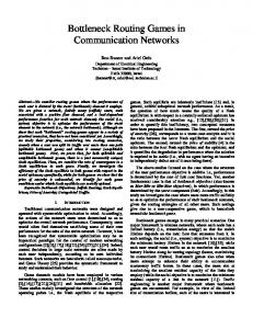
Radioactive Material DOE: defines by strategic significance
DOT: defines by process or use
Specific
Class 7: Radioactive Material *
Fissile
HLRW
Special Nuclear Material
Spent Fuel
Category I "high"
Category II "moderate"
Category III "low"
Definitions are not exclusive at these levels. * Note: not all subclasses of Class 7 are shown.
Figure 2.1: Regulatory Classification of Radioactive Materials definitions. Often, Memoranda of Understanding among these agencies clarify regulatory responsibilities and resolve problems caused by different definitions. Figure 2.1 shows how radioactive materials are defined by each agency. Legal definitions for each of these materials, as found in the U.S. Code of Federal Regulations (CFR), are included in Appendix 1. Using Figure 2.1, one can interpret the overall regulatory framework under which radioactive shipments are made. For example, fissile materials are classified as a Class 7: Radioactive Material by the DOT and are subject to regulations specific to fissile materials as well as the general Class 7 regulations. Moreover, because Class 7 is one of the nine hazard classes of hazardous materials (49 CFR 177.8), fissile materials are also subject to general hazardous material regulations. Furthermore, if the fissile material shipment includes a certain amount of plutonium and/or uranium, it is also considered a special nuclear material and subject to either Category I, II, or III regulations. In summary, in order to locate regulations applicable to a particular
radioactive shipment, one must determine (1) all of the classifications to which the material belongs, and (2) the departments that are responsible for regulating the shipment. The scope of regulatory authority of radioactive transportation can be summarized as “prescribing regulations for safe transportation of hazardous materials in intrastate, interstate, and foreign commerce” (DOT General Regulatory Authority, 49 U.S.C.A. §5103). In 1996, these regulations included requirements for radioactive material route selection, registration (shipping papers, placarding, marking, and labeling), minimum driver requirements, vehicle inspection, inspectors to monitor transportation operations, etc. Some of these regulations, like uniform placarding, marking, and labeling, are not controversial because they are seen as promoting safe and efficient nuclear material transportation. These uniform rules provide a body of knowledge that can be understood, referred to, and relied upon by shippers, carriers, drivers, emergency personnel, and law enforcement officials (Mullen 86). Other regulations, like minimum training for drivers or emergency
4
restrictions to total bans. As increasing numbers of local ordinances appeared, government and industry became concerned that nuclear material transportation would be stopped or greatly restricted on a national basis. HM-164 regulations, authorized under the Hazardous Materials Authorization Act, addressed this problem by providing a nationally-uniform highway routing system for radioactive materials. These regulations also gave the DOT regulatory authority to preempt inconsistent state and local regulations (Mullen 86). The finalized HM-164 regulations, which are primarily codified at CFR 173.22 and 177.825 state, “a carrier or any person operating a motor vehicle that contains a radioactive material for which placarding is required ... shall (1) ensure that the motor vehicle is operated on routes that minimize radiological risk; (2) in determining the level of radiological risk, consider available information of accident rates, transit time, population density and activities, and the time of day and day of week during which transportation will occur; and (3) tell the driver which route to take and that the motor vehicle contains radioactive materials” (49 CFR 177.825). These criteria do not apply when there is only one practical highway route available or when the truck is operated on preferred roads (defined below) such that the route is chosen to minimize time-intransit. Time-in-transit is further defined in 49 CFR 177.853 which states that while in transit, there is to be no unnecessary delay from and including the time of commencement of loading the cargo until its final discharge at the destination. There are two ways in which roads become part of the transportation system for placarded shipments of radioactive materials. At the federal level, HM-164 regulations define all interstate as “preferred roads” except those that travel directly through a city.
response personnel, are controversial only when defining what “minimum” requirements should be and who should finance the training. Of all the regulations, those applicable for route selection are probably the most controversial. The first DOT regulations that established a nationally-consistent highway routing system for radioactive materials, HM164 regulations, were proposed in 1978, finalized in 1981, and upheld in court in 1984. These regulations raise important underlying issues concerning the degree of involvement and responsibilities of state and local governments in regulating the movement of radioactive materials (Mullen 86). Because many of these issues remain unresolved, routing regulations are discussed in detail below. Prior to 1976, routing designations that limited or restricted the movement of radioactive materials over highways were not common. On January 15, 1976, highway shipments of spent research reactor fuel from Brookhaven National Laboratories in Long Island were blocked from traveling through the City of New York by an amendment in the city’s health code. Low-level radioactive materials were allowed entry without advance notification but were required to be transported over specified truck routes. Highlevel radioactive materials required a Certificate of Emergency Transport that was issued only “for the most compelling reasons involving urgent public policy or national security interests transcending public health and safety concerns” (Mullen 86). Following the enactment of the New York City Code, numerous state and local jurisdictions passed similar ordinances restricting or banning nuclear material shipments. By 1982, more than 200 state and local governments had enacted some form of regulations on certain shipments of radioactive materials. These regulations ranged from time-of-day travel
5
Although it is desirable to minimize the risk and travel time associated with a radioactive material shipment, a route that uses only preferred roads may not achieve either of these objectives. For example, sometimes two preferred roads may not intersect each other, but be connected by a short non-interstate connector (Hill 93). In these cases, the state could enhance safety and improve the operational efficiency of the transportation system by legally designating the connector as an “alternate” preferred road (which is really an “additional” road in the sense that it does not replace an interstate link but augments the transportation system). The requirement that routes be selected to minimize time in transit may also lead to poor routing decisions because the multiobjective nature of the radioactive routing problem is not explicitly recognized, e.g., the least-time, least-cost or shortestdistance routes may not correspond the leastrisk route. For example, one study related to hazardous material shipments by railroad found that population exposure, one component of risk, could be reduced by 20 to 50 percent by re-routing at an increase in traffic circuitry cost of 15 to 30 percent (Glickman 83). In a case filed in 1988,a similar concern was raised in regard to radioactive material shipments. The case arose because HM-164 regulations did not state how shippers were to select nonpreferred roads needed to pick-up and deliver shipments. The DOT Administrative Law Judge in the case ruled that a carrier may select road links used to pick-up or deliver materials on the basis of reducing radiological risk even though the link may be longer. Subsequently, Docket HM-164C was adopted in May 1990 to ensure that HRCQ radioactive materials are transported to and from preferred roads to pickup or delivery sites via the shortest distance. It also provided means for calculating permissible deviations for
In the latter case, an interstate beltway, if available, is to be used in place of interstate located within the beltway (49 CFR 177.825). However, if a state believes that a primary or secondary road link may be safer than a specific interstatelink, it can ban through shipments on the interstate link by legally designating the primary or secondary road link as an “alternate preferred road.” In order to compare risk among road links, states may use guidelines prepared by the DOT that are published in Guidelines for Selecting Preferred Highway Routes for Highway Route Controlled Quantity Shipments of Radioactive Materials or Guidelines (US DOT 89). A current list of alternate preferred roads and the interstate links they replace is found in the DOT’s Research and Special Program Administration’s computerized Hazardous Materials Information Exchange (HMIX) (Ardila-Coulson 94) which can be can be accessed via Internet at hmix.dis.anl.gov. As of January1997, seven states (Arkansas, Colorado, Iowa, Kentucky, Nebraska, Tennessee, and Virginia) had replaced interstate links with alternate preferred roads (Hill 93). Other states have used Guidelines but found that the risk index computed for the proposed alternate road was comparable to that for the interstate link it could replace. A carrier is allowed to deviate from preferred roads for three reasons: (1) to rest, refuel, and repair the vehicle; (2) to pick up, deliver, or transfer a regulatory-defined “highway-route-controlled-quantity” (HRCQ) radioactive material; and (3) to avoid emergency conditions that make continued use of the preferred road unsafe or impossible. Although emergency conditions are not explicitly defined in regulations, they have been interpreted to include those caused by adverse weather and traffic situations (Mullen 86).
6
proposed roads was in an area of rapid growth and high development (Ardila-Coulson 91). In order to compare risk among routes, many states use the DOT’s Guidelines report, which separates the different components of risk into two categories. Primary factors consider radiation exposure from normal (accident free) transportation, public health risk, and economic risk from accidental release of radioactive materials (ArdilaCoulson 91). If a similar risk index is computed for proposed road links using formulas that consider these primary factors, which implies that a unique least-risk road link cannot be identified, Guidelines recommends using secondary factors to select the safest road link. Some of these secondary route comparison factors include emergency response activities, evacuation procedures, avoidance of special facilities such as schools and hospitals, and avoidance of routes with higher traffic fatalities and injuries (ArdilaCoulson 91, US DOT 89). Initial experience in selecting preferred routes tends to indicate that population is highly correlated with the least-risk road link. For example, Maryland used the Guidelines to compare Interstate 95 and US 301 and the preferred road link selected was the one with the least population (Ardila-Coulson 90). While the routing criteria for HCRQ radioactive shipment center on the dual objectives of minimizing risk and maintaining departure time and scheduling flexibility, those for strategic nuclear materials and some classifications of radioactive materials such as irradiated reactor fuel and spent nuclear fuel (SNF) are very different. Because these materials can be used to create nuclear weapons, the fundamental routing objective is to protect a shipment from theft and sabotage attempts, especially within populated areas (10 CFR 73.25, 10 CFR 73.37). This objective impacts not only the basic nature of route selection and scheduling processes, but
cases that would minimize radiological risk to the public (Hill 93). For example, if a shipper wants to use a road link with lower radiological risk that is longer than the shortest-distance link, it cannot exceed five times the length of the shortest-distance pickup or delivery link (49 CFR 177.825). The case reaffirms one of the fundamental challenges of formulating regulations governing the selection of routes for radioactive shipments, namely, that criteria used to select routes are often conflicting and, optimized as a single objective, lead to different routing decisions. From a legal perspective, the nationallyuniform highway system for radioactive materials reflects a compromise between a shipper’s right to transport these materials without undue burden on commerce and a local government’s right to protect the health of its citizens (Mullen 86). For example, by banning curfews, the departure and scheduling flexibility of shippers is maintained. By restricting the number of roads that may be used to transport these materials, concentration of personnel and financial resources available for emergency response activities is possible. A distinction should also be made regarding the implied intent of regulations at the federal and state levels. One of the main objectives only found at the federal level is to prevent undue burden on commerce. States, on the other hand, are responsible for analyzing the multiple components of risk and determining whether or not primary or secondary road links are safer than interstate links. States have this responsibility in order to incorporate local knowledge of risk on specific roads while maintaining a regional perspective of the problem. For example, public hearings held in Nevada about the selection of an alternate road link for HRCQ radioactive shipments revealed that one of the
7
be notified a priori of shipments of special nuclear materials that travel in or through the governor’s state. Prenotification includes, among other things, the origin and destination of the shipment and the seven-day periods during which the shipment is estimated to depart, arrive at state boundaries, and arrive at the final destination. This notification is either mailed at least seven days in advance of the shipment’s departure or sent via messenger at least four days in advance. If the announced schedule cannot be met, the licensee is to telephone the governors and inform them of the extent of the delay beyond the schedule originally reported. If the shipment is canceled, a cancellation notice is sent to the governors (10 CFR 71.97). Advance notification is done primarily for emergency response awareness and to ensure that local law enforcement authorities along the route of a shipment are ready to respond to an emergency call for assistance (10 CFR 73.26). Prenotification also gives states the opportunity to use local law enforcement officers to escort shipments through their jurisdictions at their own cost (Doman 93, Blalock 93). Other means by which shipments are protected from theft and sabotage attempts include using escorts and specialized communications as well as monitoring the status and position of the shipment. Escorts and specialized communication are used to provide early detection of a terrorist attack that may occur when the shipment is being transported or during personnel shift changes that occur en route. For example, when transferring a shipment, at least five armed personnel must protect the shipment and two of the armed personnel are to monitor the location remotely. The remote location may be a radio-equipped vehicle or a nearby place, apart from the shipment area, so that a single act cannot remove the capability of the personnel protecting the shipment from
the methodological requirements needed to solve for an optimal least-risk route. In particular, two new problems can be identified. The first concerns the need for a priori planning and scheduling of shipments in order to ensure that arrangements have been made for local law enforcement authorities along the route of a shipment to respond to an emergency call for assistance – particularly theft or radiological sabotage attempts (10 CFR 73.26). The second routing problem recognizes that a real-time routing strategy may be needed to quickly identify the best route for transporting a shipment to a secure location if a theft or sabotage attempt is suspected. A priori planning activities include route selection and shipment scheduling. Roads that may be used to transport strategic nuclear materials are distinct from those used to transport HRCQ shipments. Specifically, regulations state that all shipments of strategic nuclear materials are to be made on primary highways with minimum use of secondary roads (10 CFR 73.25). This routing regulation is probably due to terrorism concerns and the need to select routes that do not travel through major cities during the day. Shippers are also to select routes that avoid areas of natural disaster or civil disorders such as strikes or riots (10 CFR 73.25). Some route scheduling criteria for strategic nuclear materials are similar to those for non-strategic nuclear materials, such as transporting material without unnecessary delay and without intermediate stops except for refueling, rest, or emergency stops. Other route scheduling criteria are specific to the objective of minimizing theft and sabotage attempts. These include scheduling shipments to avoid following regular patterns and preparing detailed route plans for advance notification purposes (10 CFR 73.25). Advance notification refers to the requirement that the governor of a state must
8
DOE in the late 1980’s to track shipments of radioactive materials including spent fuel, high-level waste, transuranic waste, and other high visibility shipments as determined by the DOE. TRANSCOM uses technologies of navigation, satellite communication, computerized database management, user networks, and ground communication with en route shipments (US DOE 89). Icons showing the position of the vehicle can be displayed on a series of computer-generated maps. Three levels of geographic detail are available to the user: the entire U.S., an individual state, or an individual county. The icon is color-coded green, yellow, magenta or red to show the status of the vehicle. A shipment that is proceeding normally is indicated by a green icon. A yellow icon indicates there is a problem such as a mechanical breakdown, flat tire, etc. A more serious problem, not yet affecting safety, is displayed by a magenta icon. If the vehicle is involved in an accident or in other emergency situations, a red icon is displayed (Johnson 94). Additionally, TRANSCOM contains information about individual shipments that is useful in the event of an emergency. This information includes the schedule, planned route, type of radioactive material, and required emergency response actions. Furthermore, in the event of an accident, a specific agency, the Joint Nuclear Accident Coordinating Center, offers assistance in incidents involving nuclear weapons, weapons components, and DOE-owned radioactive materials (US DOE 89). An illustration of how these requirements impact route selection and scheduling is found in Doman’s and Tehan’s (93) recount of spent fuel and irradiated hardware shipments to and from the General Electric (GE) Morris Facility. GE was involved with some of the first SNF shipments by rail in the 1980’s. Preshipment activities included a notification letter,
calling for assistance. Furthermore, each of the armed escorts and other armed personnel are able to maintain communications with each other. The commander has the capability of communicating with the personnel at the remote location and with local law enforcement agencies for emergency assistance. While in transit, the commander is to call the remote monitoring location at least every 30 minutes to report the status of the shipment. If the calls are not received within the prescribed time, the personnel in the remote location are to request assistance from the law enforcement authorities and notify the shipment control center (10 CFR 73.26). This specialized communication system also provides the opportunity for the remote monitoring location to communicate alternate itineraries en route as conditions warrant (10 CFR 73.25). In order for law enforcement authorities to respond as quickly as possible to an emergency, the status and position of the shipment are monitored (10 CFR 73.26). Although regulations do not specifically state that this monitoring is to be performed in real time, several literature sources suggest that the DOE and DOD use real-time tracking devices. For example, since the late 1970’s the DOE and DOD have developed several real-time tracking devices that allows intense oversight, monitoring, and emergency preparedness for materials of high strategic value. These systems include SECOM III, the Naval Ordinance Tracking System (NOTTS), and TRANSCOM. SECOM III was developed in 1979 to monitor classified shipments of nuclear material via the use of military satellites. NOTTS, which was first developed in the early 1980’s, has evolved into the Defense Transportation Tracking System (DTTS) which tracks high explosives (Allen 91). TRANSCOM is a 24-hour tracking and two-way satellite communications device developed by the
9
is no specific requirement to do so (Doman 93). In summary, routing of strategic nuclear materials differs from non-strategic nuclear in two fundamental ways. First, a priori planning and scheduling of shipments and the ability to adhere to schedules becomes important in order to plan for emergency preparedness and a quick response to a sabotage attempt. Thus, a routing and scheduling model should incorporate the time-dependent and stochastic properties of travel times. As Hill (93) states, the selection of routes that will reduce time in transit is highly dependent upon factors such as the sophistication of the routing model used and assumptions made about average speeds, effects of congestion, and other variables. Alternate routing times may also be particularly sensitive to speed and traffic flow volumes by time of day (Brogan 85). Second, given that the DOE can monitor the position of a strategic nuclear shipment and communicate alternate itineraries en route, routing models that incorporate real-time information could be used to quickly identify the best route for transporting a shipment to a secure location if a theft or sabotage attempt is suspected.
containing up to ten individual shipment schedules, that was sent to affected parties. All of this scheduling and departure time information was classified and protected from public disclosure until ten days after completion of a shipment. (Specifically, 10 CFR 73.21 states that routes and quantities of spent fuel are not held from public disclosure and that schedules for spent fuel may be released after the last shipment of a series occurs. Due to national security interests, this disclosure does not apply to strategic nuclear materials). Once a notification was sent out, the schedule was not changed. If a shipment could not be made within a six-hour time frame, the shipment was canceled. For any delay in shipment of more than two hours, GE provided notification to the affected parties via coded telephone messages. While this delay notification was not required by 10 CFR Part 73, the extra communication helped all parties to keep abreast of potential changes in the schedule. This helped with any subsequent reallocation of personnel if a shipment was canceled. Of 109 shipments, 37 were canceled due to a variety of reasons. The most common reason for inability to make a shipment was transportation equipment failure. Of these, two shipments were canceled due to unexpected activation of the vehicle disabling device, which “did in fact work very well.” There were five cancellations due to weather, e.g., ice, snow, fog, or bitter cold. Other scheduling and routing activities mentioned by Doman and Tehan (93) include the use of armed escorts, chase vehicles, and pre-arranged personnel shift changes that occurred en route. GE’s shipments also involved participation from the public. For example, upon discussions with the Tri-State Tollway I94, a request was made that all shipments be scheduled to occur at low traffic times, namely sometime between 1 a.m. and 4 a.m. GE complied with the request although there
2.2.2
Other Routing Criteria Considered by the DOE In addition to criteria specifically outlined in regulations, the literature contains examples of other DOE routing considerations. These criteria include, among other things, quantification of low-probability high consequence events, avoidance of populated areas and areas with inadequate emergency response capabilities, and consideration of public opinion. This section discusses how these factors influence route selection. The DOE examines a broad spectrum of low-probability high consequence events.
10
Graphical displays of the response units were created using a geographic information system. Results of the analysis enabled identification of critical areas along a proposed highway route corridor for radioactive materials. Based on examination of a proposed highway link in Nevada, they find that critical areas, defined as having response times greater than 30 minutes, were located only in rural areas (Parentela 94). In 1995, a similar emergency response analysis tool, the Transportation Emergency Response Management (TERM), was being developed at Rensselaer Polytechnic Institute for the DOE. TERM seeks to identify existing emergency response resources, estimate response times, and determine deficiencies in the existing emergency response system (Orzel 95). Finally, public perception of risk may have a significant impact on both route selection and safe transportation of radioactive materials. As mentioned previously, the ability of citizens to identify conditions that make specific transportation links unsafe allows the federally defined radioactive material transportation network to be sensitive to local health and safety concerns. However, public perception of risk may also be disruptive to shipments. As Freudenburg (91) states, if people perceive a problem to be real, it will be real in its consequences, whatever the official pronouncement may be. For example, some researchers have examined the effects of unintentional shipment stoppages on risk. Shipments stopped en route may increase the public’s radiological exposure, a function of travel time and population characteristics, especially those stoppages occurring in urban areas (Baughman 91). Unintentional stoppages of a radioactive material shipment may generate considerable publicity and reinforce the public’s doubts about the reliability of transportation operations.
For example, Salidi et. al. (91) evaluated the sufficiency of highway bridges for nuclear fuel transportation and Trask (91) looked at implications of asteroid and comet impact on SNF and high-level radioactive materials. Studies have also been conducted to determine tradeoffs between routing through densely populated and sparsely populated areas. Densely populated cities do not want shipments on their highways because of high development while small cities cite proximity to housing and schools and lack of emergency response capabilities as reasons not to ship on their highways (Ardila-Coulson 91). Credible scenarios of worst case transportation accidents in highly developed urban areas suggest that public perception of risks and area stigmatization could produce economic effects on the order of several million dollars (Baughman 91). Moreover, the Federal Railway Administration reported that the criterion of most significance to normal transportation risk appears to be the percentage of population in urban, suburban, and rural density zones and length traveled in each of the three population density zones (US DOT 91). These attributes are used by the DOE in RADTRAN to compute risk along a predetermined highway route (Neuhauser 92). These studies support arguments to select routes for radioactive materials that avoid populated areas. However, it is important to recognize the potential negative consequences of an accident involving a radioactive material release in a rural community unprepared to deal with an emergency situation or respond to a theft attempt of strategic nuclear materials. For example, Parentela et. al. (94) evaluated the emergency response capabilities of first responders, specifically fire services, within the State of Nevada. They examined the general capabilities of emergency responders, their jurisdictions, and response times.
11
Moreover, severe accidents may confirm the public’s worst fears; even a severe accident in which cask integrity is maintained may be a source of apprehension rather than comfort (Glickman 91). As a result, the DOE must consider how public fears and NIMBY (not in my back yard) sentiments can draw attention to and unknowingly endanger shipments. For example, Doman and Tehan (93) cite GE’s experience in shipping SNF by rail through St. Paul, Minnesota, between 1 a.m. and 3 a.m. Initially, shipments had media coverage and protesters present. Only after extended passage of time and the onset of bitter cold weather did the protesters and media lose interest in the SNF shipments. This is one example of how public perception may be disruptive to the safe transportation of SNF. In summary, although the perception of the broader public and their ability to assess risk often reflects more wisdom than was once apparent (Freudenburg 91), NIMBY sentiments persist.
routes may not be the same, they can have different shipping costs. Several models have looked at operational costs associated with these different types of “optimal” routes. One of the first models to explore differences among minimum risk, minimum accident likelihood, and minimum truck operating cost routes was developed by Saccomanno and Chan (85). Their model investigates tradeoffs among these criteria based on three singleobjective analyses. Through examining the transportation network in Toronto, Ontario, they find that the minimum cost strategy favors expedience at the expense of safety (List 91). Several other researchers have examined the impact of safety on cost. However, in the context of special nuclear material shipments, transportation cost appears to be a secondary, if not a negligible, factor. For example, each safe secure trailer (SST) used to transport strategic nuclear materials costs three million dollars (Kirby 96). This would lead one to conclude that compared to the high investment cost, operational costs are not as significant. This can also explain why cost is rarely used by the DOE as a routing criterion. The academic and professional communities have also indicated the need to route HAZMAT based on some measure of risk equity. Routing based on the principle of equity seeks to realize social justice by distributing risk throughout the transportation network. Essentially, risk equity techniques minimize global risk to a community while maintaining desired levels of equity between zones (Gopolan Modeling 90). Based on focused discussions with members of different interest groups affected by SNF shipments, Keeny (88) discovers that fairness and equity are viewed differently by government and public interest groups. For example, representatives from the government expressed concern for the equity between
2.2.3
Other Routing Criteria Considered in the Literature The literature also contains routing criteria researched primarily by the academic and professional communities. Most of these criteria concern transportation of hazardous materials (HAZMAT), however, many are also applicable to radioactive shipments. In general, researchers have been more concerned with cost and equity issues. They have also given more attention to the multiobjective, time-dependent, and stochastic characteristics of the radioactive material routing problem which has spurred methodological developments in these areas. This section discusses how these concerns have translated into routing criteria for radioactive material shipments. Because the optimum minimum-risk, minimum-distance, and minimum-travel time
12
impacts on present and future generations and felt that those benefiting from the generation of nuclear power should more appropriately bear the risk associated with spent fuel management. A separate criterion concerned the appropriate liability and compensation for individuals who suffered due to cancer from radiation exposure or a traffic accident with a vehicle transporting SNF. In addition to these components of risk equity and fairness, pubic interest groups expressed concerns about the psychological impacts of SNF transportation and felt that fears and anxieties that might be induced by a spent fuel management system should be considered in evaluating management alternatives. However, a decision made by the Supreme Court regarding the National Environmental Policy Act stated that fear is not an observable environmental impact (Mullen 86), which legally implies that because psychological impacts are not measurable, they do not have to be explicitly considered in route selection. A third concern of researchers is the influence of time-dependent and stochastic properties of travel times and population characteristics on the selection of an optimal least-time or least-cost route. Even methods used to estimate population densities along routes can impact route selection. For example, Sathisan and Chagari (94) find that population density estimates are sensitive to which level of spatial data aggregation (e.g., block, block group, census track, or county) is used to calculate them.
Risk = (Accident Probability) X (Accident Consequence). Instead of using accident probabilities, accident/incident rates are commonly calculated. Accident/incident data show numbers of reported accidents and/or spill incidents over specified periods. When coupled with some measure of exposure like truck-miles, these data can be used to estimate accident/incident rates. Principal difficulties associated with creating specific estimates include: (1) selecting from the set of reported accidents/incidents those which represent relevant events for the estimate to be constructed; and (2) recognizing the uncertainty in the estimates as a result of both the small numbers of accidents/incidents in specific categories, and the probable underreporting of incidents (List 91). This section discusses these issues and the impacts inaccurate rates may have on determining safe routes for radioactive shipments. Calculation of accident rates for a particular routing scenario can be complicated because accident rates can vary for a number of reasons. For example, Glickman (88) examined variations of release accident rates by mode, carrier type, vehicle type and road/track classification. Based on 1982 U.S. data, he finds that release accident rates of for-hire tank trucks are about 50 times greater than those of private tank truck carriers. Another study conducted by Saccomanno and Chan (85) looked at variations in all truck accident rates by time of day (day or night) and weather/pavement conditions (dry or wet). Based on Canadian data, they found differences were highly dependent on roadway type. For example, low-speed urban arterials had rates that were less for wet and night conditions while expressway ramps had rates that were less for dry and day conditions. Harwood, Viner and Russell (90) also looked at truck accident rates for HAZMAT routing.
2.2.4
Problems Encountered in Selecting Minimum Risk Routes DOT’s Guidelines contains criteria for selecting alternate routes based on a minimum-risk objective where risk is determined for individual route segments by the equation:
13
to avoid the possibility of a civil or criminal penalty. Because there are few inspectors to ensure compliance, the costs of compliance are often greater than those of infrequent penalties. For example, Environmental Protection Act (EPA) Region 7 officials estimate that only 10 percent of reportable releases under 100 gallons are reported to EPA, the states, or the Nuclear Regulatory Commission (NRC) if the substance released is not extremely hazardous. If the material is extremely hazardous, it would probably be reported if five gallons were spilled (Abkowitz 88). As a result, underreporting can significantly alter accident and release estimates, particularly in underestimating small incidents. However, in regards to strategic nuclear materials, the DOE maintains that the containers used to transport these materials are the primary means of protecting the public and the environment from releases (Portsmouth 90). The Transportation Management Division of the DOE, responsible for overseeing transportation of DOE-owned materials, emphasizes its excellent safety record. For example, studies show that there is a significant difference in accident risk between transporting spent fuel and transporting other energy-related commodities. In terms of statistical likelihood of fatalities, the shipment of gasoline, propane, and chlorine is from 300 to 30,000 times riskier than the shipment of all materials associated with the nuclear fuel cycle (Yu 85). Moreover, the SSTs used to transport plutonium pits are seen as 10 to 100 times safer than any other vehicle. A DOE report estimated that in the worst case scenario, the number of deaths associated with transporting plutonium pits from disarmed nuclear warheads to an interim storage facility would be caused by a very improbable traffic accident; or, in other words, deaths due to a potential release were considered to be
Their research examined accident rate differences on roadway type and area type (urban and rural) based on data on three states’ highway geometry, traffic volume, and accidents (Harwood 90). Their estimates reinforce Federal Highway Administration studies that indicate the probability of a HAZMAT release given an accident involving a HAZMAT-carrying truck vary markedly with the type of accident. For example, Abkowitz et. al. (84) derived expected release rates for eight container classes and found that the expected release fraction per mile shipped ranged from approximately 10E-8 to 10E-6. These are some examples of the difficulties associated with creating useful accident rates for events that occur infrequently and appear to have a large random component. Other concerns have been expressed about the accuracy of the current risk assessment model presented in the DOT’s Guidelines. For example, Harwood et. al. (90) charge that the default values of accident rates used are based on out-of-date accident predictive models that are 20 to 25 years old. The models also use accident rates for all vehicle types (which are primarily passenger car accidents) rather than for truck accident rates and implicitly assume that all accidents are equally likely to result in a HAZMAT release. Based on these perceived deficiencies, they propose revisions of the Guidelines. Another major problem that affects the accuracy and usefulness of accident and release rates is the underreporting of incidents. In a report prepared for the Office of Technology Assessment, Abkowitz and List (88) explore the degree of underreporting in HAZMAT transportation. They estimate underreporting to be as high as 30 to 50 percent. One reason they cite for high underreporting is a voluntary spill reporting system in which the incentive for reporting is
14
negligible (Kirby 96). Therefore, in regards to SST shipments, factors affecting the safety of shipments other than traffic accidents like catastrophic events and terrorism are prioritized.
travel time) between two points. HIGHWAY has been used to plan and schedule shipments of classified nuclear materials and to verify that carrier-suggested routes for HRCQ radioactive materials meet all DOT routing requirements (Joy 94). The HIGHWAY network database represents all of the nation’s interstate highways and most federal and major state highways. These highways are defined as links between nodes. There are more than 20,000 links and 13,000 nodes in the data set. Several types of routes can be selected using HIGHWAY including paths for the shortest travel time or distance and paths that conform to HM-164 routing regulations. HIGHWAY provides specific route, time, and distance information for each route generated. The model also has the capability to calculate alternate routes, and generate routes that avoid any specified link(s) or node(s) or a particular state or population center. Population data for the various links can be calculated for use in risk assessment models like RADTRAN (Johnson Highway 93). Future updates planned for HIGHWAY include incorporation of Transportation Emergency Response Management (TERM), integration of GIS software into routing and system analysis techniques, and ACCIDENTPROB, a model that allows the user to determine the probability of a transportation accident on a specified transportation link or section using historical accident rates and link-specific physical characteristics. A multiobjective routing model developed at Cornell University is also being modified for incorporation into HIGHWAY (Orzel 95). There are three limitations to be aware of when using HIGHWAY. First, HIGHWAY selects routes independently of risk. After initial routes are selected, RADTRAN or similar risk assessment tools like Transportation Individual Centerline Dose (TICLD) or Transat can evaluate risks on individual routes (Neuhauser 92). Also,
2.3 ROUTING MODELS Several models have been developed to select routes for radioactive materials based on one or more of the above criteria. In general, models used by the DOE are based on a single deterministic criterion or a weighted sum of multiple criteria. Route selection is almost always performed independently of risk assessment. Several researchers have proposed multi-criteria models with stochastic attributes, including models to select routes using risk as an explicit factor. This section is divided into two parts. The first describes models used by the DOE and state agencies and the second discusses models reported in the published literature, including multiobjective stochastic models. 2.3.1
DOE and State Agency Routing Models In response to HM-164 regulations, two routing models were developed by Oak Ridge National Laboratory under the sponsorship of the DOE. These models, HIGHWAY and INTERLINE, are the official DOE routing models (Joy 94). Several other models have been used by the DOE or state agencies. These include StateGEN and StateNET that were developed by the Transportation Technology Center at Sandia National Laboratories. This section describes these models and gives examples of how they have been used to examine routing issues specific to radioactive material transportation. HIGHWAY is a computerized highway routing model that determines routes by minimizing the total impedance (expressed as a weighted combination of distance and
15
the day. Population densities are computed according to a methodology detailed in Durfee’s and Coleman’s (83) report Population Distribution Analyses for Nuclear Power Plant Siting (Johnson 97). First, the area of block group polygons are calculated so that a population density can be determined. Next, a 15-second by 15-second latitude/longitude grid cell matrix is overlayed over the block group polygons and a population density is calculated for each grid cell matrix. The formula used to calculate the population density for each grid cell considers the population densities of the grid cell and its adjacent neighbors (Johnson 97, Durfee 83). INTERLINE is a computerized routing algorithm almost identical to HIGHWAY except that is determines routes for other modes of transportation including rail, barge, and air (Johnson Interline 93). StateGEN is a routing model designed to assist users in developing highway networks that address local concerns about the transportation of radioactive materials. The model allows users to create a network of roads by defining nodes that are highway intersections on the network and by identifying links that are the segments between the nodes. Once the network has been created, a dictionary file is developed to list the attributes (up to 30) of interest to the user like accident rates, population density, etc. The user must then obtain data about each attribute and assign a numerical value to each link for each one. To select a route, the user specifies an origin and a destination point on the network and the attribute to be minimized or maximized (Ardila-Coulson 91). StateNET is very similar to StateGEN except that it allows route selection based on a weighted sum of up to 10 attributes (ArdilaCoulson 91). StateGEN and StateNET have been used in Nevada for the selection of alternate preferred road links. The state collected 28
because HIGHWAY finds alternate routes by adding a penalty to all road links contained in the previous solution and running the shortestpath algorithm again, it does not guarantee that the optimal k-best routes will be identified (where optimality is defined as the least-time or least-cost paths). Second, HIGHWAY assumes that travel time and population densities are static. However, these assumptions may not be valid for longdistance shipments, especially those that travel through several major cities. In HIGHWAY, travel times are computed as the distance of a highway link divided by the posted speed limit on that link (Orzel 95). Newer versions of HIGHWAY, such as Version 3.3, have the ability to set maximum vehicle speed, (this construction is awkward) i.e., although the posted speed limit on a link may be 65 mph, the maximum speed of a vehicle can be set below 65 mph (DOE 97). The total time required to transport the shipment is a function of how many drivers are present. For two drivers, the program assumes they travel continuously for four hours and then rest for 30 minutes (Orzel 95). Newer versions of HIGHWAY can also modify the time between breaks and duration of breaks; however, changes apply consistently throughout the route. For example, a two-driver team must drive for x hours and rest for y minutes, drive for x hours, rest for y minutes, ..., until the final destination is reached (DOE 97). Thus, if different maximum vehicle speeds or break times are desired for different travel legs of a route, individual runs must be created for each travel leg. HIGHWAY cannot explicitly model the effects of congestion on travel time for a major city or recognize that the time required to travel through a large city with congestion is a function of a shipment’s departure time. HIGHWAY also assumes that population densities are constant throughout
16
attributes for 173 segments that were connected by 133 intersections. The identification of alternate preferred road links was determined by minimizing a weighted sum of four primary attributes that were equally weighted: population density, total accident rates, truck accident rates, and distance. Once the routes were selected, meetings with all bordering states were held to ensure that alternate preferred road links would be acceptable to them (Ardila-Coulson 91).
this method does not guarantee that all nondominated paths will be found (List 91). Other methodological approaches such as that by Zografos and Davis (89) have used goal programming in order to capture both routing criteria preferences and the importance associated with selecting a route that fulfills a stated preference. While a goal programming formulation offers considerable flexibility to the decision-maker and allows examination of different routing scenarios by changing the goal attainment levels and the priority for their attainment, this approach is not guaranteed to produce non-inferior solutions (List 91). Cox (84) developed a method that uses a node-labeling technique to determine all Pareto-optimal solutions in a multiobjective HAZMAT problem with deterministic link attributes. Turnquist (87) extended Cox’s work by adding time-of-day variations in link attributes, link use restrictions, and probabilistic elements to the core algorithm. By associating a departure time label with each node, the algorithm is able to incorporate time-of-day restrictions associated with the node or with arcs emanating from the node. The label can also be used to read timedependent attributes of an arc such as travel speeds and population densities. In order to determine all non-dominated routes, a shortest-path problem is defined for each objective. For deterministic link attributes, the shortest path algorithm is run for each possible departure time and each individual objective. For stochastic link attributes, the routing algorithm is applied after sampling from distributions of the stochastic link attributes. Simulation is then used to examine the effect of stochastic link attributes on routing (Wijeratne 93). Wijeratne, Turnquist, and Mirchandani (93) extend this approach to develop a method for approximating stochastic dominance among paths with uncertain values. They apply their Stochastic,
2.3.2
Other Routing Models Presented in the Literature List et. al. (91) provide an excellent synopsis of HAZMAT routing models. This section summarizes a few of the models discussed in their article in order to provide an overview of methodological approaches developed for examining how route selection is affected by multiple objectives or the timedependent and stochastic properties of risk and travel time. Two particular applications of routing models emphasized in this section include risk equity and curfews. (a) Overview of Some Single-Criterion and Weighted Multiple-Criteria Models Similar to the HIGHWAY algorithm, early routing models typically used standard linear programming techniques to optimize an objective function consisting of a single criterion or a weighted combination of multiple criteria. Some models that use these techniques include those by Robins (83) and Saccomanno and Chan (85). However, because they compare criteria based on separate single objective analyses, their method of analysis does not provide any explicit information about tradeoffs among various criteria. Complete analysis of tradeoffs is also not possible when a weighted combination of criteria is optimized because
17
Multiobjective Shortest Path (SMOSP) to the routing of HAZMAT materials in the AlbanySchenectady-Troy area of New York State. As reflected in these models, the academic and professional communities have been concerned with multiobjective, timedependent, and stochastic characteristics of the HAZMAT and radioactive routing problem. Relationships among departure time, travel time, and risk have also been explored. Two other concerns expressed in the literature include risk equity and curfew restrictions.
maximum differences in risk that exist between two zones, where the sum is taken over the trips made. They formulate their model as an integer programming problem and as a dynamic programming model and use heuristic methods to determine upper bounds for large scale problems. (c) Curfews One of the interesting policy issues surrounding curfews is that, while reducing risk for those cities imposing time-of-day restrictions, they might simultaneously increase risk in other communities. Indeed, during the HM-164 hearings, one of the main arguments raised by shippers was that transportation would be greatly restricted by curfews passed by local governments that did not consider the entire radioactive material transportation system (Mullen 1986). Although locally-imposed curfews were officially banned after the HM-164 hearings, routing analyses which incorporate curfews can be beneficial to citizens and shippers. For example, although curfews passed by local governments with narrow regional perspectives are not feasible, curfews based on national guidelines that consider global risk versus shipper cost may be warranted. Moreover, even if curfews are not formally mandated, shippers can benefit from using a routing model that schedules a shipment’s departure time and breaks so as to minimize delays and operational costs due to congestion in large cities. Thus, to model curfews, two new problems arise. The first is an operational consideration: for a carrier facing a particular set of curfews in specific cities, the shipper desires to schedule shipments so as to minimize total transit time, including delay due to the curfews. Second, for policy analysis it is important to be able to analyze the aggregate effects of curfews such as (1) estimating the total delay added to travel time
(b) Risk Equity One of the limitations identified in early HAZMAT routing models is that they did not consider certain important aspects of risk, such as equity. Later papers address this issue by seeking to minimize global risk to a community while maintaining desired levels of equity between zones. Early modeling approaches to the risk equity problem such as that by Zografos and Davis (89) formulated the problem as a capacitated assignment problem by associating capacity constraints with arcs. Gopolan, Batta, and Karwan (Gopolan Equity 90) formulate the problem by defining distinct zones in the transportation network. The optimal path is defined as the one that minimizes global risk subject to the constraint that the maximum difference in risk between any pair of zones is below a specified bound (List 91). This idea was later extended to finding a set of routes between a single origin and destination that satisfies the same criteria (Gopolan Modeling 90). Linder-Dutton, Batta, and Karwan (Linder-Dutton 91) point out that if a set of routes is to be used to achieve risk equity, ordering of these routes should maintain some measure of equity after a fewer number of routes have been taken. They propose an “equitable sequencing problem” that minimizes the sum of the
18
due to vehicles stopping to avoid violating curfews and (2) identifying how the spatial distribution of risk may change. Also, as Cox (86) states, when determining how curfews affect risk, it is important to remember that because delays caused by curfews could increase total time en route, they also increase some elements of risk. Some research has addressed the scheduling of shipments in the presence of curfews. For example, Cox and Turnquist (86) examined curfew delay for a fixed route and deterministic travel times and looked at the impact of stochastic intercity travel times. Using Cox’s and Turnquist’s assumptions, when given a departure time and a fixed route, an optimal strategy that minimizes total in-transit time delay time is to delay a shipment only when it is about to violate a curfew and to delay it only until the curfew passes. Since this procedure yields the minimum delay solutions for any specified departure time, the departure scheduling problem can be solved by a simple enumeration scheme. By repeating this analysis for various possible departure times, the variation of delay with respect to the departure time can be plotted, as illustrated in Figure 2.2 (Cox 86).
However, intercity travel times for hazardous materials shipments may have a large random component that should not be ignored in scheduling decisions. To account for these, the authors derive a recursion to estimate the expected delay given the departure time of the shipment to obtain a probability distribution for intercity travel times. By comparing deterministic and stochastic models, the authors are able to make several general conclusions. First, the random travel time analysis indicates that the best departure times are not as good as the deterministic model predicts, and that the worst times are not as bad. Given greater uncertainty of arrival times for points further along the route, it becomes difficult to plan a departure time for a precise arrival for points located further from the origin. Second, the authors find that for any given number of cities imposing a curfew, the variance in total shipment delay is large, indicating that the total delay is sensitive to which cities impose curfews (Cox 86). 2.4 SUMMARY AND MAJOR CONCLUSIONS Depending on the class of radioactive materials, different routing strategies may be more applicable. For example, for placarded shipments of radioactive materials that are not of strategic significance and do not require escorts, one of the most important unresolved routing issues involves the shippers’ right to transport without undue burden and local and state governments’ right to protect the health of their citizens. Because the main intent of HM-164 regulations (as interpreted by the courts) was to implement a standardized highway routing system for radioactive materials, it did not prioritize risk minimization, especially on a jurisdiction-byjurisdiction basis (Mullen 86). Therefore, it may be warranted to (1) examine how alternate risk-minimization routing strategies
Curfew Delay (hrs)
12 8
4
0 12
3 6 9 12 3 6 AM AM AM PM PM
9 PM
12
Departure Time
Figure 2.2: Curfew Delays as a Function of Departure Time
19
routes. The next chapter presents a timedependent least-cost path algorithm that can be used to analyze how time-dependent travel times and population densities, curfews, and waiting impact radioactive material route selection and departure flexibility.
such as avoiding cities during rush hour impact the selection of routes and the number of optimal departure time windows, and (2) compare the relationships among local risk, global risk, and economic costs for these alternate routing criteria. However, for shipments of strategic nuclear materials, economic cost is not the primary consideration. Instead, protection of the shipments from theft and sabotage are of primary concern. Both a priori planning and real-time routing activities can help protect a shipment. As stated in 10 CFR 73.25, in order to minimize the vulnerability of strategic nuclear material shipments, one should do the following: (1) pre-plan itineraries, (2) periodically update knowledge of route conditions, (3) maintain knowledge of the status ad position of the materials while en route, and (4) determine and communicate alternate itineraries en route as conditions warrant. Pre-planning routes and itineraries are important for emergency response awareness. Pre-notification ensures that arrangements have been made for local law enforcement authorities along the route of shipments to respond to an emergency call for assistance, particularly theft or radiological sabotage attempts. Although these regulations do not mention that activities (2) and (3) should occur in real-time, up-to-date knowledge of route conditions and vehicle location can enable real-time routing strategies that may be most appropriate and most warranted given suspicious terrorist activities or sabotage and theft attempts. Finally, regardless of the routing strategy developed, several data quality issues are applicable. One of the most important issues involves the calculation of population density and travel times that are used as primary route comparison factors. Models that take into account time-of-day population changes and travel times may find different minimum risk and minimum travel time
20
the TDLCP allow consideration of curfews on major cities or waiting at safe havens. This chapter describes the TDLCP algorithm and extensions applicable to radioactive material transportation. The mathematical formulation and algorithmic solution framework of a time-dependent leastcost path problem with extensions to curfews and waiting at node are first presented. Next, modifications made to the more general TDLCP algorithm, and implemented in this study, are discussed. An example problem is given to help visualize the steps of the modified algorithm.
3. TIME-DEPENDENT LEAST-COST PATH ALGORITHM 3.1 INTRODUCTION As discussed in the background review of Chapter 2, routes must be selected and/or schedules must be prepared before radioactive and strategic nuclear materials are transported. These a priori activities help ensure that safe routes are selected and that local emergency response and law enforcement personnel can respond quickly to a radioactive material release or an attempt to steal or sabotage the shipment. In order to comply with the U.S. Code of Federal Regulations, shippers must select a route that minimizes time in transit and/or the number of people who will be exposed to the shipment along the route. Current routing and scheduling models used by the Department of Energy (DOE) for strategic nuclear material shipments assume travel times and population densities are constant. However, this assumption may lead to the selection of an inferior route, especially for shipments that travel through several major cities. As an example, consider the difference in travel times and population densities for a shipment that might travel through New York City at 2 a.m. versus 5 p.m. Thus, in order to accurately analyze risk and select the route that is in compliance with Federal guidelines, it is important to be able to model the time-dependent characteristics of travel times and population densities. To include time-dependent travel times and population densities in routing and policy analyses, the time-dependent least-cost path (TDLCP) algorithm developed by Ziliaskopoulos and Mahmassani (93) for Intelligent Transportation Systems (ITS) applications can be modified. This algorithm provides more flexibility and policy sensitivity than current models used by the DOE which were discussed in the preceding chapter. For example, simple extensions to
3.2
GENERAL FORMULATION OF THE TDLCP PROBLEM This section describes the mathematical formulation of the TDLCP problem and introduces notation and definitions that are used throughout the chapter. A summary table of these definitions is included in Figure 3.13 at the end of the chapter for easy reference. The problem of interest is to find the optimal route and departure time for a radioactive material shipment from a given origin node to a destination node for a transportation network in which the travel times and/or costs are time-dependent. Imposing curfew restrictions on cities or allowing a shipment to wait at a safe haven is also permitted via modifications to the TDLCP algorithm. The problem is formulated as a one-toall shortest path problem, in which it is required to find the time-dependent shortestpaths from a given origin to all destinations in a network for all desired departure times. A directed transportation network with nonnegative arc costs and a discrete time scale, G = (V, A, T), is assumed, where V is the set of nodes, A the set of arcs, and T the set of time intervals in the network. The discrete time scale is discretized into time intervals of
21
length δ. Travel times and costs on the arcs are defined in multiples of the positive time δ for every time step of the discrete scale T = {t0 , t0 + δ, t0 + 2δ, ..., t0 + mδ}where t0 is the earliest departure time from the origin node, δ is a small time interval during which a perceptible change in travel time and/or costs occurs, and m is large integer such that t0 + mδ is the latest possible arrival time at the destination nodes. Tij(k) represents the nonnegative time to travel from Node i to Node j when departing from Node i during time interval k and Cij(k) represents the nonnegative cost associated with departing from Node i during time interval k to travel to Node j. Because time has been discretized, it is assumed that travel times and costs remain constant during time δ. Formally, these assumptions are expressed as Tij(τ) = Tij(t0 + kδ) and Cij(τ) = Cij(t0 + kδ) for every τ in the interval t0 + kδ < τ < t0 + (k +1)δ. Because strategic nuclear materials are often transported long distances, the total travel time can be in excess of 24 hours. Thus, for the general radioactive shipment problem, Tij(k) can be defined for all discretized time intervals in a 24-hour period, or for k = {1, 2 , ..., mod(1440/δ +1)} where δ is expressed in minutes and 1,440 is the number of minutes in 24 hours. This notation assumes travel times are constant from day to day; however, if desired, differences in average weekday and weekend travel times could be captured by expanding the definition of k. In order to read the proper travel time within this 24-hour framework a function p(k) is defined for time interval k and is equal to k - mod(k/(1440/δ)) x 1440 x δ. Thus, the travel time between Node i and Node j for time interval k is generally given as Tij(p(k)). Finally, although most of the transportation network is composed of rural Interstate highways in which the travel times remain constant over the day, a small value of δ
should be used to reflect changing travel times in suburban and urban areas. To use a label-correcting method to solve for the time-dependent shortest paths from the origin to all nodes in the network for all departure time intervals, time and cost label vectors are associated with each node. In order to more clearly relate these labels to how they are implemented in the TDLCP code, four indices are now introduced. Specifically, when a vehicle departs Node i during time interval k it arrives at downstream Node j at time interval l. When no waiting at a node is permitted in the network, the time of departure at Node j is always equal to its time of arrival. Thus, if a vehicle arrives at Node j during time interval l, it also departs during time interval l. It is through modifying the definition of index l that curfews and waiting are modeled in the TDLCP algorithm. Using the notation currently defined and assuming no curfews or waiting occurs in the network, a time label, λj(l), is used to store the arrival time of a vehicle traveling from the origin that arrives at Node j during time interval l. Time labels are also used to read the correct arc costs and ensure the proper progression of time through the network. Similarly, a cost label, ηj(l), stores the cumulative cost associated with a shipment that travels from the origin and arrives at Node j during time interval l. Each node has a time and cost label for every time interval in the period of interest. Formally, the vector of time labels, Λj, is expressed as {λj(t0), λj(t0 + δ), ..., λj(t0 + (m -1)δ)}, while the vector of cost labels, Hj, is equal to {ηj(t0), ηj(t0 + δ), ..., ηj(t0 + (m -1)δ)}. In each iteration of the TDLCP algorithm, Node i is scanned when temporary cost and time labels are calculated for nodes located downstream of Node i for each time interval of interest. The temporary cost label computed for downstream Node j at interval l contains the value of the current least-cost
22
path representing a vehicle that travels from the origin and arrives at Node j during time interval l (which also travels through Node i during time interval k). The temporary time label represents the time the shipment arrives at Node j when taking this path. In order to use a label-correcting method to find the shortest paths, the mathematical formulation of two steps is required in order to (1) compute temporary cost and time labels, and (2) compare temporary and current cost labels and decide whether or not to update current cost and time labels. Two implementation issues affecting the efficiency of the algorithm are discussed in the next section and include: (1) how nodes having the potential of improving the current shortest path are identified, and (2) which data structures are used to represent the network and store the optimal least-cost paths. In order to use cost and time labels to find the optimal least-cost paths, all cost labels are first initialized to infinity, except labels at the origin node that correspond to desired departure times. These latter labels are initialized to zero. All time labels are initialized to zero except labels at the origin node that are initialized to desired departure times. At any computation step in the TDLCP algorithm, the vector of cost labels, Hj, will be equal to infinity or the value of the current least-cost paths for a vehicle that departs from the origin node and arrives at Node j during time interval l. Time labels, Λj, contain values equal to zero, desired departure times, or the time of arrival at Node j corresponding to the least-cost path from the origin node. When a vehicle departs from Node i during time interval k and travels to downstream Node j, the temporary cost label for Node j is calculated as the sum of the current cost label for Node i for time interval k and the cost to travel on arc (i,j) when departing from Node i during time interval k. Formally, this is given by ηi(k) + Cij(k).
Cost and time labels are updated when a temporary cost label computed for downstream Node j is less than the current cost label assigned to that node. The temporary cost label is compared to the current cost label of downstream Node j for the time interval the vehicle arrives at Node j, which has been defined as interval l. Formally, interval l is given by mod{{λi(k) + Tij(k)}/δ}+ 1. Upon termination of the algorithm, cost labels at the destination nodes will either be equal to (1) infinity (indicating that no feasible path exists for a vehicle to arrive at the destination node during time interval l for the given departure time constraints) or (2) the least-cost path from the origin node that arrives at the destination node during time interval l. The minimum cost label for a destination node vector is the least-cost path from the origin to that destination. The departure time and path corresponding to the optimal cost are found by tracing back through the network from the destination node to the origin node via a path pointer array. This array is described in the next section. Finally, because interstate shipments of radioactive materials may travel in different time zones, an origin node may not be located in the same time zone as a destination node. As a result, all departure and travel times should reference a base time, such as midnight Eastern Standard Time (EST). Also, because certain parameters, such as the start of a curfew period in a city, may be a function of the city’s time zone, an integer time zone label, TZ(i), is assigned to every node to indicate in which time zone Node i is located. Eastern Standard Time (EST), which is used as the reference time zone, is represented by TZ(i) equal to one. Likewise, a node in the Central Time Zone will have a time zone label equal to two, and a Mountain Time Zone node and a Pacific Time Zone node will have labels equal to three and four, respectively. Using
23
these indicators, a function can now be defined to calculate how much time-zone dependent factors need to be “shifted” from the base time zone. Formally, this function, defined as TZshift(i) for Node i, is equal to (TZ(i) - 1) x 60 when time is expressed in minutes. For example, if Cstart is used to denote the start of a curfew period that occurs during the morning rush hour period and references midnight EST, then the proper Cstart parameter for Node i’s time zone is Cstart- TZshift(i) for all nodes i in which the morning curfew applies.
labels and how they find the least-cost paths. For example, while a label-setting algorithm designates one label as permanent at each iteration, a label-correcting algorithm considers all labels as temporary until the final step. Therefore, a label-setting algorithm will converge on the least-cost path as soon as the destination node label is assigned whereas the label-correcting algorithm finds the least-cost path only after all nodes having the potential of improving the distance labels have been scanned (Ahuja 93). Because of the manner in which labelsetting and label-correcting algorithms find the shortest path, theoretically the former is more efficient in terms of worst case computational complexity (Ahuja 93). However, actual performance on any given problem depends greatly on the specific implementation as well as the specific problem. Data structures such as the deque scan eligible list can be used to exploit special characteristics of time-dependent transportation networks, allowing labelcorrecting procedures to outperform label setting ones on transportation networks (Ziliaskopoulos 93). Finally, it is important to note that in the context of time-dependent shortest-path and time-dependent least-cost problems, another limitation of a label-setting algorithm can arise. Specifically, because the labelsetting algorithm implicitly assumes that the first-in first-out (FIFO) property holds on all arcs of the network, the algorithm can fail to detect the optimal path in a time-dependent network (Ziliaskopoulos 93). In a timedependent least-time path (TDLTP) problem, the FIFO property can be interpreted as “the sooner a vehicle departs from Node i the sooner it arrives at downstream Node j.” Similarly, in a TDLCP problem, the FIFO property can be interpreted as “the sooner a vehicle departs from Node i the less it costs to
3.3 IMPLEMENTATION ISSUES FOR THE TDLCP ALGORITHM This section first motivates the use of a label-correcting procedure to solve for the set of optimal paths from an origin to all destinations in a network with time-dependent travel times and/or costs. Three implementation issues are described in order to detail the algorithmic steps of the TDLCP algorithm and explain how the TDLCP algorithm is able to operate efficiently by exploiting special characteristics of timedependent networks. These implementation issues include network representation, data structure of the scan eligible (SE) list, and path storage. 3.3.1
Motivation for Using A LC Algorithm to Solve a TDLCP Problem Shortest-time or least-cost path problems are generally solved by label-setting (LS) or label-correcting (LC) algorithms that use an iterative approach to assign temporary time and/or cost labels to nodes at each step. In the TDLCP problem, the cost label, ηj(l), is an estimate or upper bound on the least-cost path from the origin node to Node j for a vehicle arriving at Node j during time interval l. Label-setting and label-correcting algorithms differ in how they update their cost
24
travel to downstream Node j.” Thus, the FIFO property assumes that no benefit is gained by waiting at Node i. However, this may not be the case for time-dependent networks or for networks where waiting at nodes is not penalized. In order to correctly solve for the optimal time-dependent path using a label-setting algorithm, non-FIFO arcs can be transformed using a transformation proposed by Ziliaskopoulos (92). In summary, because of the flexibility and efficiency possible with a label-correcting procedure, the TDLCP algorithm proposed by Ziliaskopoulos and Mahmassani (93) was modified for the radioactive material routing and scheduling problem of interest in this study.
to, Node i. The forward star representation uses a concept similar to that of node adjacency list. Denoting the set of arcs (i,j) in a network as A, the node adjacency list of Node i can be expressed as the set of nodes j for which (i,j) ∈ A. Thus, for the network shown in Figure 3.1, the adjacency list of Node 1, A(1), is Node 2 while the adjacency list of Node 2, A(2), includes both Nodes 3 and 4. To identify when all elements of a list have been read, the last element in the list is assigned the value of zero. Thus, if the only entry in a node’s adjacency list is zero, no arcs emanate from that node. A complete node adjacency list for the example network in Figure 3.1 is shown in Figure 3.2. 3
3.3.2
Forward Star Network Representation Several data structures may be used to store the topology of a network, information associated with the network’s arcs and nodes, and intermediate results. Although the representation used to store, maintain, and update the network can play a significant role in the performance of an algorithm, no data structure is superior for all algorithms and for all problems. Instead, the most efficient algorithm for solving a problem is often superior because its data structure exploits the unique characteristics of the problem. In the case of the TDLCP problem, a forward or reverse star network representation used in a label correcting procedure with a deque scan eligible list has been proposed because of its efficiency and generality (Ziliaskopoulos 93). The forward star representation stores the topology of a network by identifying those nodes immediately downstream, or adjacent
1
2
5 4
Figure 3.1: Network for Adjacency List and Forward Star Example Node(i)
Adjacency list A(i)
i=1
1
2
0
i=2
2
3
4
i=3
3
5
0
i=4
4
5
0
i=5
5
0
0
Figure 3.2: Node Adjacency List for Example Network
25
N=5
Tail node node(i)
Pointer fstar(i)
Head node node(j)
i=1
1
1
2
i=2
2
2
3
i=3
3
4
4
i=4
4
5
5
i=5
5
6
i=6
6
6
M=5
tail
head
5
Figure 3.3: Forward Star Representation for the Example Network By assigning a pointer, fstar(i), to each i, Node the forward star representation stores the node adjacency list in a single array and eliminates the need for zero entries. Using the pointer, the heads of the arcs emanating from Node i can be determined. This is because the pointer fstar(i) “points” to the index of the head node array where the first downstream node (also referred to as the head node) of Node i is located. All of the downstream nodes of Node i are stored in the head node array in indices fstar(i) to fstar(i+1) - 1. If Node i has no outgoing arcs, fstar(i) is set equal to fstar(i+1). Node i will have no outgoing arcs when fstar(i) is less than fstar(i+1) - 1. In order to maintain consistency, fstar(1) is typically set equal to 1 and fstar(N+1) is assigned a value equal to M + 1 where N is the number of nodes and M is
the number of arcs in the network (Ahuja 93). The forward star representation for the example network is presented in Figure 3.3. The forward star index can also be used to store arrays of arc data. In the TDLCP problem, both costs and travel times are stored for each arc. Travel times and costs for the arcs are defined for each discretized time interval k, where k is defined from one to the maximum number of time intervals, m. In the general TDLCP problem, a second index is added to the forward star index in order to store time-dependent travel times and costs. Figure 3.4 shows a complete representation of the network arrays used to store data for the general time-dependent least-cost problem with time-dependent travel times and costs.
Cost (i,j,k)
Tail node node(i)
Pointer fstar(i)
Head node node(j)
i=1
1
1
2
i=2
2
2
3
i=3
3
4
4
i=4
4
5
5
N=5 i=5 5 i=6
6
k=max int
k=max int
...
6 M=5 5 6
Travel time(i,j,k)
...
k=2 k=1
k=2 k=1
Figure 3.4: Network Representation for the General TDLCP Problem
26
Gains in efficiency can be seen when a forward star network representation is used in a label-correcting procedure because in each iteration temporary cost labels are calculated for all nodes downstream of Node i. By storing the network representation in a forward star pointer array, these downstream nodes can be efficiently identified. This is because the fstar pointer explicitly points to these downstream nodes which are stored in the head node array from fstar(i) to fstar(i+1).
NextNode for any time step l, the time and cost labels for NextNode are updated and NextNode is inserted into the SE list. The algorithm continues by deleting a node from the SE list, defining it as the CurrentNode, scanning each of its downstream nodes, and computing temporary cost labels for each time interval. The algorithm terminates when the SE list is empty. In order to perform these operations efficiently, Ziliaskopoulos and Mahmassani (93) adopted a double-ended queue, or deque structure for the SE list that was introduced by D’Esopo and tested by Pallotino (84). In the deque, NextNode can be inserted at the beginning or end of the one-dimensional array. If NextNode has never been in the SE list before, it is inserted at the end of the SE list, otherwise if NextNode is not currently in the SE list it is inserted at the beginning of the list. Thus, a node is always in one of three states: (1) currently in the SE list, (2) previously in the SE list but not there now, or (3) previously not in the SE list and not there now. In order to determine the state of Node i and its position in the SE list, the deque array associates a number with each node according to the following definition:
3.3.3
Scan Eligible (SE) List In a label-correcting algorithm, an SE list is used to store those nodes that have the potential of improving the labels of at least one other node. During the initialization stage of the algorithm, only the origin node is in the SE list. In the first iteration, the origin node is deleted from the SE list and defined as the CurrentNode. When no waiting occurs at the CurrentNode, the temporary cost labels for all adjacent downstream nodes of CurrentNode are then calculated as ηi(k) + Cij(k) for each time step k. The interval associated with these temporary cost labels corresponds to the time interval the vehicle arrives at the downstream node which (was previously defined as interval l). If the temporary cost label, CostTemp, for downstream node NextNode is less than the current cost label of Deque(i) =
-1 if Node i has been in the SE list but is not there currently
0
if Node i has never been in the SE list
j
if Node i is currently in the SE list where j is the node next to it in the list
∞ if Node i is the last node in the SE list
27
Finally, two pointers are defined for the SE list: FirstNode points to the first node in the list and LastNode points to the last node. By inserting nodes which have previously been in the SE list at the beginning of the list, the deque structure captures the fact that if the label of NextNode changes, then the downstream nodes of NextNode updated in previous iterations will likely change as well. Thus, instead of continuing to update nodes downstream of both nodes, by inserting NextNode at the beginning of the list fewer iterations will typically be required to find the optimal paths.
The steps of the general TDLCP algorithm can be summarized as: STEP 1: INITIALIZE (a) Create the SE list and initialize it by inserting into it the origin node. (b) Initialize the cost label vectors by setting Hj = (∞, ∞, ..., ∞) for j = 2, 3, ..., N and H1(k) = 0 if k ≤ mod(departure time/δ) +1 < k + 1 and infinity otherwise for all departure times and k = 1, ..., m. (c) Initialize time labels to zero by setting Λj = (0, 0, ..., 0) for j = 2, 3, ..., N and Λ1(k) = departure time if k ≤ mod(departure time/δ) +1 < k + 1 and zero otherwise for all departure times and k = 1, ..., m. (d) Initialize path pointers NodePoint(j,l) and IntPoint(j,l) to infinity for j = 2, 3, ..., N and l = 1, ..., m. Also initialize NodePoint(1,l) and IntPoint(1,l) to zero if l ≤ mod(departure time/δ) +1 < l + 1 and infinity otherwise for all departure times and l = 1, ..., m.
3.3.4
Path Storage In order to determine the route and departure time corresponding to an optimal path solution, both the upstream node of Node i and departure time from the upstream node must be maintained. To store this information, a two-dimensional pointer array is defined for each node. This array has length m, or an entry for each time interval in the routing problem. In the pseudo-code and example problem presented later in this chapter, NodePoint(j,l) stores the upstream, or predecessor, node of a vehicle that arrives at Node j during time interval l. IntPoint(j,l) stores the interval corresponding to the time the vehicle departed the predecessor node in order to arrive at Node j during time interval l. The use of path pointers to find the optimal departure time from the origin node corresponding to the minimum least-cost path at a destination node d is described in Section 3.5.
STEP 2: SCAN (a) Select the first Node i from the SE list, name it CurrentNode, and delete it from the list. d IF the SE list is empty, THEN go to STEP 4.
(b)
3.4 STEPS OF THE GENERAL TDLCP ALGORITHM This section describes the steps of the general TDLCP algorithm. A discussion of the steps and pseudo-code detailing how these steps are implemented are also included in this section.
Otherwise, define the set of nodes located downstream of Node i as Γ{i}and scan the CurrentNode, Node i, according to the following equation for all k time steps: Hj(l)
28
= min { Hj(l), Hi(k) + Cij(k) } for j ∈ Γ{i}
where: Hj(l)
=
Hi(k)
=
Cij(k)
=
l
=
correspond to allowed departure times that are initialized to zero. For implementation purposes, infinity is defined as a large number greater than the maximum cost for a route. All time labels are initialized to zero except labels at the origin node that are initialized to allowed departure times. All path pointers NodePoint(j,l) that are used to store to the upstream, or predecessor, node of a vehicle arriving at Node j during time interval l are initialized to infinity except for those intervals at the origin corresponding to the potential set of feasible departure time intervals that are initialized to zero. Likewise, all path pointers IntPoint(j,l) used to store the interval corresponding to the departure time of a vehicle at the predecessor node are initialized to infinity except for those origin nodes corresponding to allowed departure time intervals. These latter labels are initialized with the allowed departure times. By defining the set of desired departure times from EarlyDepart to LateDepart and DeptTime the time between successive departures, the following pseudocode shows how this initialization step can be achieved:
Cost label of downstream Node j at time interval l Cost label of CurrentNode, Node i, at time interval k Cost of traveling from Node i to Node j when departing from Node i during time interval k Time of arrival at downstream Node j when leave Node i during time interval k
(c) IF Hj(l) is greater than Hi(k) + Cij(k), THEN insert CurrentNode into the SE list. STEP 3: ITERATE (a) Repeat STEP 2. STEP 4: STOP (a) Terminate the algorithm. The mdimensional vectors Hj contain the costs of the time-dependent shortest paths from the origin node to every Node j in the network.
FirstNode = 1 LastNode = 1
3.4.1
Discussion of the Initialization Step During the initialization stage, the SE list is created by inserting the origin node into the list and assigning initial values of deque(i) to each node. This is done by initializing FirstNode and LastNode to 1, (where Node 1 has been defined as the origin node). Deque(i) is initialized to zero for all nodes except for deque(1) which is set equal to infinity. Also during this stage, the cost labels, time labels, and path pointers are initialized for all N nodes for all m time intervals. All cost labels are assigned values of infinity, except labels at the origin node that
deque(1) = infinity DO (for all nodes i, i = 2, N) deque(i) = 0 DO (for all nodes i and all time intervals k) Cost(i,k) = infinity Time(i,k) = 0 NodePoint(i,k) = infinity IntPoint(i,k) = infinity DO (for desired departure times k, k=mod(EarlyDepart/DeptTime) + 1 mod(LateDepart/DeptTime) + 1) Cost(1,k) = 0 Time(1,k) = (k-1)*DeptTime NodePoint(1,k) = 0 IntPoint(1,k) = k
29
Next, these procedures are incorporated into pseudo-code presented for all of Step 2.
3.4.2
Discussion of the Scanning Step After initialization, the TDLCP algorithm begins by deleting the first node from the SE list and defining it as CurrentNode. Next, CurrentNode is scanned by computing temporary cost and time labels for all downstream nodes for all k time intervals. In each iteration, the algorithm computes two temporary labels: CostTemp is the cost of departing from CurrentNode for downstream node NextNode at Time (CurrentNode, k), and TimeTemp is the corresponding arrival time at NextNode. For ease of readability, the corresponding time interval of TimeTemp was defined as interval l. If the current cost label Cost (NextNode, l) is greater than CostTemp, Cost (NextNode , l) and Time (NextNode, l) are updated by being replaced by CostTemp and TimeTemp, respectively. The path pointers for the predecessor node and time interval are also updated by setting NodePoint (NextNode, l) equal to CurrentNode and IntPoint (NextNode, l) equal to k. If, for any iteration, a label of NextNode is updated, NextNode is inserted into the SE list. After all downstream nodes having the potential of improving the least-cost shortest path have been inserted in the SE list, the algorithm continues by repeating Step 2. The algorithm terminates when CurrentNode is equal to infinity, which indicates that the SE list is empty. To code the LC algorithm, several intermediate procedures can be defined. These include procedures to delete a node from the SE list, insert a node into the SE list, and compute temporary cost and time labels. The latter step is explained as a separate procedure because it is in this step that most of the modifications for the extensions to the TDLCP algorithm occur. In order to visualize the scanning step, these intermediate procedures are first detailed and pseudo-code for them is given.
(a) Deletion of a Node from the SE List During the deletion procedure, the first node of the SE list is deleted from the SE list and assigned as CurrentNode. In order to perform the deletion procedure, CurrentNode, the SE pointer FirstNode, and the deque label for the node being deleted must be updated. These steps are executed as follows: CurrentNode = FirstNode FirstNode = deque(CurrentNode) deque(CurrentNode) = -1
(b) Insertion of a Node into the SE List In order to insert NextNode into the SE List, the state of NextNode and the value of SE pointers FirstNode and LastNode must be known. NextNode is inserted in the SE list only if deque(NextNode) is equal to -1 or 0. If deque(NextNode) is equal to -1, indicating that NextNode has been previously been in the SE list but is not there currently, it is inserted into the front of the SE list through changing the FirstNode index and deque(NextNode) label. This is accomplished via the following steps: deque(NextNode) = FirstNode FirstNode = NextNode
If deque(NextNode) is equal to 0, indicating that NextNode has never been in the SE list, it is inserted into the back of the SE list. If there are no nodes currently in the SE list when NextNode is inserted in the list, both the FirstNode and LastNode pointers must be updated along with the deque label for NextNode. Otherwise, only the LastNode pointer and deque label for NextNode need to be updated. Formally, this can be implemented as:
30
IF ( deque(NextNode) = 0 and FirstNode = infinity ) FirstNode = NextNode LastNode = NextNode deque(NextNode) = infinity
(d) Complete Pseudo-Code for Scanning Step The DELETION, INSERTION, and LABEL procedures detailed above are used in the scanning procedure as follows:
ELSE IF ( deque(NextNode) = 0 and FirstNode ≠ infinity ) LastNode = NextNode deque(NextNode) = infinity
DO 1 WHILE CurrentNode ≠ infinity (or, do while the SE list is not empty) CALL DELETION of first node from SE list
ENDIF
DO 2 for all nodes downstream of CurrentNode NextNode = downstream node for which temp labels are to be computed InsertInSEList = FALSE
(c) Computation and Use of Temporary Cost and Time Labels Using an embedded loop structure, temporary cost and time labels are computed for each downstream node at each time interval. The calculation of cost and time labels when no waiting at nodes is permitted is summarized as:
DO 3 for all time intervals k CALL LABEL for (NextNode, l) to compute and compare cost label for downstream node at time interval l
CostTemp = Cost(i,k) + Cij(k) TimeTemp = Time(i,k) + Tij(k) l = mod(TimeTemp/δ) + 1
3 CONTINUE IF InsertInSEList = TRUE CALL INSERTION of NextNode in the SE list
Once temporary cost and time labels have been computed, the temporary cost label is compared to the current cost label Cost (NextNode, l). If CostTemp is less than Cost (NextNode, l), the cost label, time label, node path pointer, and interval path pointer for Node NextNode at time interval l are updated. A Boolean indicator, InsertInSEList, is also set to TRUE to indicate that NextNode should be inserted in the SE list if it is not there already. Formally, the comparison of temporary cost and time labels is:
2 CONTINUE 1 CONTINUE
3.5 EXTENDING THE TDLCP ALGORITHM TO FIND OPTIMAL DEPARTURE TIMES This section describes how path pointers, which are used to store the optimal least-cost path corresponding to each time interval at the destination nodes, can also be used to find optimal departure times from the origin node that correspond to the minimum of the least-cost paths found for a specific destination. To find the departure time at the origin node, Node 1, corresponding to the optimal shortest path for a particular arrival time interval at a particular destination node, path pointers NodePoint(j,l) and IntPoint(j,l) are
IF (Cost(NextNode, l) > CostTemp) Cost(NextNode, l) = CostTemp Time(NextNode, l) = TimeTemp NodePoint(NextNode, l) = CurrentNode IntPoint(NextNode, l) = k InsertInSEList = TRUE ENDIF
31
used. In this notation, indices j and l are used to denote the fact that the optimal shortest path and corresponding departure time from the origin for a given arrival interval at a destination node are found by “tracing back” along the path to find the preceding Node i and time interval k from which a vehicle departed in order to arrive at Node j during time interval l. For an arrival time occurring in interval l at destination node d this can be accomplished via the following steps:
NodePoint (1,k) was initialized to zero for all intervals k corresponding to desired departure times. In order to find the optimal departure times from the origin corresponding to the minimum least-cost path for all D destination nodes, a preliminary loop is added and slight modifications are made to the basic implementation structure detailed above. The preliminary loop is used to first scan the cost labels at the destination nodes in order to (1) find the value of the minimum least-cost paths for each destination node and (2) store the arrival time intervals for each destination node that correspond to the minimum leastcost paths for that destination node. The basic implementation structure is then modified to iterate over all these optimal destination node arrival time intervals for each destination node in order to find the corresponding optimal departure times at the origin node. Formally, the value of the minimum least-cost paths for all D destination nodes and the arrival time intervals at Node d corresponding to this minimum least-cost path are found via the following steps:
STEP 1: INITIALIZE (a) Initialize NodeTemp to d and IntTemp to l. STEP 2: TRACE (a) IF NodeTemp = 0, THEN go to STEP 4. (b) ELSE find the preceding node and interval by defining NodeTemp2 = NodeTemp and updating NodeTemp to NodePoint(NodeTemp, IntTemp) and IntTemp to IntPoint(NodePoint2, IntTemp).
STEP 1: INITIALIZE (a) Initialize LeastCost (d) to infinity and define a one-dimensional vector to store how many optimal arrival time intervals correspond to the minimum least-cost paths for destination Node d as OptIntCount (d). Set OptIntCount (d) to zero for all D destination nodes. (b) Initialize a two-dimensional array, OptInt (d,k), used to store the arrival time intervals at departure node d that correspond to the minimum least-cost paths at that destination node, to infinity for all D destination nodes and k time intervals.
STEP 3: ITERATE (a) Repeat STEP 2. STEP 4: STOP (a) Terminate the algorithm. The optimal departure time interval corresponding to the optimal leastcost path at the destination node d for time interval l has been found and is equal to IntTemp. The optimal departure time is given by Time(1,IntTemp) where Node 1 has been defined as the origin node. To clarify, this extension to the TDLCP algorithm is able to detect that the optimal departure time from the origin has been found when NodeTemp = 0 because
32
3.6 FORMULATION OF THE TDLCP PROBLEM WITH CURFEWS AND WAITING This section describes two extensions of the TDLCP algorithm that can be used to model practical routing considerations and analyze policy questions related to radioactive material transportation. In the first extension, curfews are incorporated in order to analyze how a set of curfews imposed on cities affects departure time flexibility when no waiting is allowed along the route. These curfews are modeled both as hard and soft constraints. As hard constraints, no violation of curfews is permitted and a route that violates a curfew will never be selected. In order to determine the minimum number of curfews a shipment encounters for a given departure time, curfews are also modeled as soft constraints. The second extension of the TDLCP algorithm permits a shipment to wait at certain locations along a route such as at “safe havens.” In a network with curfews, safe havens can also be used as places for a shipment to wait instead of traveling though a city during a curfew period. Waiting allows analysis of another policy question associated with curfews, namely, how does waiting en route reduce the number of people who are exposed to the shipment while increasing total travel time and shipment costs? In the problem formulation, it is assumed that curfew cities and waiting locations are not the same. However, if the same node is both an involuntary (i.e., curfew) and voluntary waiting location, this can be modeled by creating two nodes connected by a virtual arc with zero cost and zero travel time. Similar to the previous section, the mathematical formulation is first presented followed by a discussion of the specific implementation steps.
STEP 2: IDENTIFY MINIMUM LEAST-COST PATH FOR EACH DESTINATION NODE (a)
Compare the current value of LeastCost(d) to the Cost label for destination Node d for all k time intervals for all D destination nodes. Update LeastCost(d) according to the following: LeastCost(d) = min{ LeastCost(d), Cost(d,k) }
STEP 3: STORE OPTIMAL ARRIVAL TIME INTERVALS AT DESTINATION NODES (a)
Store the optimal arrival time intervals corresponding to the minimum least-cost path for each destination node by updating OptInt(d,k) according to the following relationship for all k time intervals for all D destination nodes: IF Cost(d,k) = LeastCost(d) ≠ infinity THEN OptIntCount(d) = OptIntCount(d) + 1 OptInt(d,OptIntCount(d)) = k ENDIF
The basic structure used to find the optimal departure time from the origin node corresponding to a specific least-cost path at a particular destination node and particular destination arrival time interval can now be extended to iterate over all D departure nodes and optimal arrival time intervals at destination Node d which are given by OptInt(d,OptIntCount(d)). Upon termination of the algorithm, the optimal departure times at the origin corresponding to the minimumleast cost paths for each destination node will be found.
33
account for the fact that a shipment may arrive at downstream node, NextNode, during its curfew period if NextNode is a city in which a curfew is observed. By always storing the departure time and departure time interval in path pointers and redefining index “l” as the time of departure from Node j, TimeTemp and CostTemp labels can be modified to reflect the cost and time of waiting at downstream node NextNode. The correct calculations of CostTemp and TimeTemp are also dependent on in which time zone NextNode is located. In a given iteration of the standard TDLCP algorithm, the cost and time labels for downstream node NextNode when departing from CurrentNode, Node i, at time interval k are calculated from the following steps:
3.6.1
Formulation of the TDLCP Algorithm with Curfews To model curfews, C curfews periods are defined and Curfew(c) denotes the subsets of cities in which curfew period c is observed for c = 1, 2, ..., C. For example, Curfew(1) ∈ V may represent the subset of cities in the network in which a morning curfew is applicable and Curfew(2) ∈ V may be the subset of cities in which an evening curfew is observed. CStart(c) and CEnd(c) represent the beginning and end of curfew period c for c = 1, 2, ..., C. Thus, CStart(1) and CEnd(1) would represent the beginning and end of the morning curfew period for all cities ∈Curfew(1) while CStart(2) and CEnd(2) would contain the beginning and end of the evening curfew period for all cities ∈Curfew(2). In order to model curfews, high arc costs can be associated with those links departing from a curfew city during its curfew period. If the arc cost is equal to infinity, the TDLCP algorithm will never select a path that enters a curfew city during its curfew period. This is because the temporary cost label calculated for nodes located downstream of the curfew city will always be greater than or equal to infinity. In this scenario, it is possible that for a given set of departure times, no feasible paths will be found. Therefore, in order to determine the minimum number of curfews a shipment encounters for a particular departure time, a high cost, less than infinity and defined as CurfewCost, can be associated with arriving at a curfew city during any of its curfew periods. In this case, the shipment can be forced to stop at the city until the end of the curfew period. In order to model curfews, the network cost structure can be modified and the standard TDLCP algorithm can be applied directly to find the optimal least-cost paths. Formally, this is done by modifying the temporary cost and time label calculations to
STEP 1: INITIALIZE TEMP LABELS (a) Calculate the arrival time and arrival time interval for downstream Node j, NextNode, for a shipment that departs Node i during time interval k by setting TimeTemp = Time(i,k) + Tij(k) and l = mod(TimeTemp/δ) + 1. (b) Also calculate the cost of traveling on this path by setting CostTemp = Cost(i,k) + Cij(k). dIF no waiting occurs at downstream node NextNode, THEN these labels also represent the departure time and departure time interval being observed for NextNode.
34
labels for downstream node NextNode for a shipment that departs Node i during time interval k when curfews are present in the network are summarized in the following pseudo-code:
STEP 2: UPDATE TEMP LABELS IF CURFEW APPLIES (a) IF NextNode ∈ Curfew(c) for c = 1, 2, ... C, THEN determine if the shipment arrives at NextNode during curfew period c by first accounting for time zone differences by defining:
TimeTemp = Time(i,k) + Tij(k) CostTemp = Cost(i,k) + Cij(k) l = mod(TimeTemp/δ) + 1
CStartTemp = CStart(c) TZShift(NextNode), and CEndTemp = CEnd(c) TZShift(NextNode). (b)
DO for all c ∈ C IF NextNode ∈ Curfew(c) CStartTemp = CStart(c) -TZShift(NextNode) CEndTemp = CEnd(c) - TZShift(NextNode)
IF CStartTemp ≤ TimeTemp < CendTemp, THEN update CostTemp to infinity and TimeTemp to CEndTemp.
IF CStartTemp ≤ TimeTemp < CendTemp CostTemp = CurfewCost TimeTemp =CEndTemp ENDIF
The only difference between these steps and the previous ones used to calculate temporary time and cost labels for NextNode is the updating of TimeTemp to CEndTemp and CostTemp to infinity if a shipment arrives at curfew city NextNode during one of its curfew periods. Essentially, by setting TimeTemp to CEndTemp, a virtual arc is created that represents a shipment that must stop at NextNode until the end of its curfew period. If soft curfew constraints are desired, CostTemp can be updated in Step 2 by setting it equal to Cost(i,k) + CurfewCost. CurfewCost could also be defined as a function of how long the shipment is forced to wait at NextNode in order not to penalize a shipment that waits 5 minutes the same as one that waits 2 hours. To determine how long a shipment has waited at a curfew node j ∈ Curfew(c), CEndTemp(c) - Time(i,k) - Tij(k) can be computed for each node j in the optimal path that is a curfew city with an arrival time Time(i,k) + Tij(k) occurring curfew period c. The algorithmic steps associated with the calculation of temporary cost and time
ENDIF
Finally, note that the same modeling concepts described above can be used to represent time windows. (A curfew identifies times at which a shipment cannot travel over a transportation link while a time window identifies times during which a shipment may travel over a transportation link.) An example application of a time window would be a toll authority that requests their roads only be traveled on during the early morning hours. 3.6.2
Formulation of the TDLCP Algorithm with Waiting The modeling of waiting at nodes is very similar to the modeling of curfews. A set of cities or places where waiting is permitted, C3 ∈V is defined. C3Max represents the longest wait for any of the cities or places in C3. Two costs are associated with waiting: C3FC(i) is the fixed cost of waiting at Node i, independent of how long the shipment waits, and C3VC(i,k) is the variable cost of waiting at Node i, i ∈ C3, k ∈ possible intervals waiting can occur, or {1, 2, ... C3MaxInt}.
35
Thus, a variable cost associated with k = 1 applies for 0 < time spent waiting at node ≤ 1δ; a variable cost associated with k = 2 applies for1δ < time spent waiting at node ≤ 2δ, etc. Different waiting times at nodes can easily be modeled by setting C3VC(i,k) equal to infinity for k greater than the maximum number of intervals waiting can occur at Node i. As with curfews, virtual arcs are created to represent waiting at nodes through modifying the temporary time and cost labels and the TimeTemp label is used to store the departure time being examined for downstream node, NextNode. However, unlike curfews, the departure time from a waiting node is not directly known and must be optimized by the TDLCP algorithm. This is done by adding another loop in the TDLCP algorithm to calculate these labels for all possible waiting time intervals that can be spent at NextNode if NextNode ∈ C3. In order to determine the amount of time spent waiting at a node in the optimal path, the path pointers and travel times are used. In order to clarify how the waiting time at Node j is calculated, the “l” index in the general TDLCP formulation is modified and a fifth index, “w” is added: a vehicle is said to depart Node i at time interval k to travel to Node j where it waits for time w before departing during time interval l. At the termination of the algorithm, Time(i,k) contains the optimal departure time from Node i that occurs during time interval k and Time(j.l) contains the optimal departure time from downstream Node j that occurs during time interval l. The path pointer for Node j at time interval l will “point” to predecessor Node i and the time of departure from that node. Using this notation, the optimal waiting time w on an optimal leastcost shortest path for Node j is given as: Time(j,l) - Time(i,k) - Tij(k). In order to find the optimal least-cost paths from an origin to all destinations in a
network and the optimal waiting times on nodes, modifications in the calculation of temporary time and cost labels are made, similar to those proposed earlier for curfews. The main difference between the modeling of curfews and waiting is that now the TDLCP algorithm itself must be modified to allow calculation of temporary time and cost labels for all possible waiting intervals. To modify the algorithm a new loop is embedded to indicate how many times the LABEL procedure should be called for downstream node NextNode, or, how many temporary time and cost labels should be calculated for waiting node NextNode after departing from CurrentNode at time during time interval k. The pseudo-code for how this loop can be implemented in the TDLCP algorithm is described after the steps for calculating temporary time and cost labels are presented. In a given iteration of the modified TDLCP algorithm, the cost and time labels for downstream node NextNode when departing from CurrentNode, Node i, at time interval k are calculated from the following steps: STEP 1: INITIALIZE TEMP LABELS (a) Calculate the arrival time and arrival time interval for downstream Node j, NextNode, for a shipment that departs Node i during time interval k by setting TimeTemp = Time(i,k) + Tij(k) and l = mod(TimeTemp/δ) + 1. Calculate the cost of traveling on this path by setting CostTemp = Cost(i,k) + Cij(k). (b) Initialize C3nInt, the number of waiting time intervals, to one and WaitTemp, a temporary label representing the time spent waiting at NextNode, equal to zero.
36
4 CONTINUE
STEP 2: UPDATE TEMP LABELS IF WAITING APPLIES IF NextNode ∈ C3, THEN set: (a) (b) (c) (d)
3 CONTINUE IF InsertInSEList = TRUE CALL INSERTION of NextNode in the SE list
TimeTemp = TimeTemp + (C3nInt -1) x δ WaitTemp = WaitTemp x (C3nInt -1) x δ WaitIntTemp = mod(WaitTemp/δ) + 1 CostTemp = CostTemp + C3FC(NextNode) + C3VC(NextNode,WaitIntTemp) for (C3nInt -1) > 0.
2 CONTINUE 1 CONTINUE
3.7 TDLCP ALGORITHM APPLIED TO THE RADIOACTIVE SHIPMENT PROBLEM This section describes how the TDLCP algorithm was modified to solve for the optimal departure times and least-cost paths for radioactive material shipments. Several unnecessary modifications were made to the general TDLCP algorithm which were described thus far. This section describes these modifications and presents an example problem in order to help visualize the steps of the TDLCP algorithm implemented in this study.
It is through initializing C3nInt to 1 and updating it to C3MaxInt only if NextNode is a city where waiting is allowed, that a loop is created in the TDLCP algorithm. This loop calls the LABEL procedure once if NextNode is not a city where waiting occurs and times if NextNode is a city where waiting occurs. C3nInt + 1 intervals are used because optimal waiting decision at NextNode may be not to wait at all (in which case TimeTemp and CostTemp are not updated as reflected in Steps 2A and 2D). Formally, this loop is implemented in the TDLCP algorithm as seen in the following pseudo-code:
3.7.1 Formulation of the Radioactive Shipment Problem In the radioactive shipment and scheduling problem examined in this study, travel times are assumed to be constant and two arc costs, Cost1(a) and Cost2(a), are defined for all arcs a ∈ A. Cost1(a) is the night-time population residing within one mile of arc a and Cost2(a) is the number of people who live or work within one mile of arc a during the day. Day costs on arcs are defined from StartDay to StartNight while night costs on arcs are defined from midnight to StartDay and from StartNight to midnight. A general cost function is defined to represent whether or not a vehicle departs CurrentNode during the day or during the night. Specifically, the cost function was defined as Cost1 if the vehicle departs from CurrentNode during the night and Cost2 if the
DO 1 WHILE CurrentNode ≠ infinity (or, do while the SE list is not empty) CALL DELETION of first node from SE list DO 2 for all nodes downstream of CurrentNode NextNode = downstream node for which temp labels are to be computed InsertInSEList = FALSE C3MaxInt = 0 DO 3 for all time intervals k IF NextNode ∈ C3 THEN C3MaxInt = mod(C3Max/δ ) + 1 ENDIF DO 4 for n = 1, C3MaxInt + 1 CALL LABEL for (NextNode, l) to compute and compare cost label downstream node when depart that node during time interval l
37
vehicle departs from CurrentNode during the day. However, it should be noted that with this TDLCP algorithm, any non-negative cost function can be used. Other possible functions for this particular application include: (1) defining cost as a proportion of the amount of time the vehicle travels on arc a during the day (Cost2 times) and night (Cost1 times), or (2) defining cost as the maximum of Cost1 and Cost2 for those arcs that have a departure time from CurrentNode in one cost interval (e.g., night) and arrival time at NextNode in the other cost interval (e.g. day). The second definition of cost is a more conservative definition. Because interstate shipments may travel in different time zones, parameters such as StartDay and StartNight need to be referenced according to a base time zone, the time zone label described in the general formulation of the TDLCP algorithm, TZ(i), is assigned to every node. Eastern Standard Time (EST), which is used as the reference time zone, is represented by TZ(i) equal to one. All time is expressed as minutes and references midnight EST. The set of possible departure times is defined from EarlyDepart to LateDepart where EarlyDepart is the earliest desired departure time, expressed in minutes after midnight and LateDepart is the latest desired departure time. Thus, the total number of departure time intervals being analyzed is equal to mod((LateDepart - EarlyDepart)/δ) + 1. These parameters also reference midnight EST. To determine the departure time that gives an optimal route over a 24-hour period, EarlyDepart is set equal to zero and LateDepart to (1440 - DeptTime) where DeptTime is defined as the amount of time, in minutes, between successive departures. By solving for the optimal path for each possible departure time, policy questions, such as the reduction in departure time flexibility when curfews are imposed, are analyzed.
Cost and time labels are updated when a temporary cost label computed for downstream Node j is less than the current cost label assigned to that node. If a vehicle departs from Node i during time interval k during the night and travels to downstream Node j, the cost label is computed according to Equation 3.1. Otherwise, the cost label is computed according to Equation 3.2 that uses the day-time cost for arc(i,j). ηi(k) + Cost1(i,j) [Equation 3.1] ηi(k) + Cost2(i,j) [Equation 3.2] In the radioactive shipment problem implemented in this study, logical functions are used to determine whether the vehicle departs from CurrentNode during the day or night in order to compute the correct cost of arriving at NextNode during time interval l. The calculation of cost and time labels when no waiting at nodes is permitted is summarized as: IF (Time(CurrentNode, k) occurs during the night for CurrentNode’s time zone) CostTemp = Cost(CurrentNode, k) + Cost1(CurrentNode, NextNode) ELSE (Time(CurrentNode, k) occurs during the day for CurrentNode’s time zone) CostTemp = Cost(CurrentNode, k) + Cost2 (CurrentNode, NextNode) ENDIF
Finally, curfews are modeled differently in the radioactive shipment problem than previously described. Because the following implementation actually modifies the TDLCP algorithm instead of modifying the network cost structure and applying the TDLCP algorithm directly, the latter is recommended for future applications. In the problem, two sets of curfew cities are explicitly defined: C1 ∈ V is the set of cities
38
ELSE IF (CurrentNode ∈ C1 or C2, k occurs during a curfew period for CurrentNode’s time zone, and the curfew period ends in CurrentNode’s night period)
in which a morning curfew is applicable and C2 ∈ V is the set of cities in which an evening curfew is observed. C1start, C1end, C2start, and C2end, expressed as minutes after midnight referencing EST, represent the beginning and end of the morning and evening curfew periods. A curfew may start and end in the same cost period or start in one period and end in the other. Unlike the previous formulation that scanned Node i and created a virtual arc for downstream Node j if Node j was a curfew city, this implementation checks to see if Node i is a curfew city and if a shipment has arrived during a curfew period. The proper progression of time in the network can be maintained by adding the time remaining until the end of the curfew onto the travel time to the downstream node. The proper cost label is calculated by determining whether the end of the curfew period occurs in the day or at night. Formally, curfews are modeled by modifying the cost and time label calculations. CostTemp and TimeTemp are now function of when the shipment arrives at Node i (e.g., does it arrive during a curfew period causing CurfewCost to apply and the shipment to be delayed?), and when the shipment departs from Node i (e.g., does Cost1 or Cost2 apply and what is the correct interval associated with the travel time of arc(CurrentNode, NextNode)?). The correct calculation of CostTemp and TimeTemp is also dependent on which time zone the CurrentNode is located in. The calculation of cost labels are now summarized as:
CostTemp = Cost(CurrentNode, k) + CurfewCost + Cost1(CurrentNode, NextNode) ELSE IF (CurrentNode ∈ C1 or C2, k does not occur during a curfew period for CurrentNode’s time zone, and Time(CurrentNode, k) occurs during CurrentNode’s day period) CostTemp = Cost(CurrentNode, k) + Cost2(CurrentNode, NextNode) ELSE IF (CurrentNode ∈ C1 or C2, k occurs during a curfew period for CurrentNode’s time zone, and the curfew period ends in CurrentNode’s day period) CostTemp = Cost(CurrentNode, k) + CurfewCost + Cost2(CurrentNode NextNode) ELSE IF (CurrentNode ∉ C1 or C2 and Time(CurrentNode, k) occurs during CurrentNode’s night period) CostTemp = Cost(CurrentNode, k) + Cost1(CurrentNode, NextNode) ELSE (CurrentNode ∉ C1 or C2 and Time(CurrentNode, k) occurs during CurrentNode’s day period)
IF (CurrentNode ∈ C1 or C2, k does not occur during a curfew period for CurrentNode’s time zone, and Time(CurrentNode, k) occurs during CurrentNode’s night period ) CostTemp = Cost(CurrentNode, k) + Cost1(CurrentNode, NextNode)
CostTemp = Cost(CurrentNode, k) + Cost1(CurrentNode, NextNode) ENDIF
39
As in its previous implementation, the temporary cost label is compared to the current cost label Cost(NextNode, l). If k does not occur during a curfew period for a curfew city, l is equal to Time(NextNode, l) + travel time from CurrentNode to NextNode at time interval k. If k occurs during a curfew period for a curfew city, l is equal to p(C1end or C2end) + travel time from CurrentNode to NextNode where p(C1end or C2end) is a function that converts the end of the curfew period into the correct ending time which may be defined over a period greater than 24 hours. Formally, this is computed as (C1end or C2end) x {mod(Time(NextNode, l)/1440) + 1} . Note that if a vehicle stops due to a curfew, the interval used to calculate the proper time label corresponds to the end of the curfew period, or mod ({p(C1end or C2end)}/DeptTime) + 1. To determine how long a shipment has waited at a curfew node for an optimal path, p(C1end or C2end) - Time(i, k) can be computed for each node in the optimal path that is a curfew city with an arrival time Time(i, k) during the curfew period.
Expressed as minutes past midnight, this would be 0 ≤ k1 < 60. The example network shown in Figure 3.5 only contains the cost and time travel data for the time intervals required to solve the problem. Figure 3.6 shows the network representation for the radioactive example, and Figure 3.7 shows the value of cost, time, and path pointer labels after the problem has been initialized. The initialization of the SE list is also seen in Figure 3.7. In this example, entries that are updated during a particular iteration are always bolded. After initialization of the example problem, five iterations of the TDLCP algorithm are required to solve for the optimal shortest path. This section illustrates how cost labels, time labels, path pointers, and the SE list are updated for each iteration. Those entries that are updated in a given iteration are bolded. Only the first iteration is explained in detail after which only significant variations from the first iteration are mentioned. In the first iteration, shown in Figure 3.8, Node 1 is deleted from the SE list and assigned to CurrentNode. The deque label for Node 1 is set to -1 to indicate the node is no longer in the SE list. Also, at this point in the iteration, note that FirstNode is equal to infinity. When Node 1 is scanned, Node 2 becomes NextNode. Temporary labels CostTemp and TimeTemp are calculated for k = 1. Because Cost(1,1) is infinity, the corresponding cost label Cost(NextNode, L) will not be updated; infinity added to the nonnegative arc cost of a(1,2) is always greater than or equal to infinity. Thus, only the cost label calculated for the desired departure time of 355, or for k = 6, will be updated. Since the vehicle departs during the night, CostTemp is equal to η1(6) + Cost1(1,2), or 0 + 10 = 10. TimeTemp is equal to λ1(6) + T1,2(6), or 355 + 30 = 385.
3.7.2 Example Problem In order to visualize the initialization procedure, consider the example network shown in Figure 3.5. In the example, assume the optimal time-dependent least-cost route is desired for a departure time of 5:55 a.m. from Node 1. Assume StartDay is 6 a.m. and StartNight is 6 p.m. and that all travel occurs within the same time zone. Thus, for 0 ≤ departure time from Node i < StartDay and for StartNight ≤ departure time from Node i < 1440 the cost on arc(i,j) is Cost1. Likewise, for StartDay ≤ departure time from Node i < StartNight the cost on arc(i,j) is Cost2. Also assume that time interval k is defined for 60 minutes. Thus, the interval associated with k = 1 extends from midnight to 1 a.m.
40
1
20 15 10
30 20 25
2
10 20
10 20 5
3 10
20 15 15 30 10 5 15
4
time k=6 k=7 k=8
30
cost Cost1 Cost2
5
40 30 5 10 10
Figure 3.5: Network for the TDLCP Example Problem
Travel time(i,j,k)
Tail node node(i)
Pointer Head node Day cost Night cost cost1(i,j) cost2(i,j) fstar(i) node(j)
i=1
1
1
2
i=2
2
2
3
i=3
3
4
4
i=4
4
5
5
N=5 i=5 5
6
i=6
6
A=5
k=max int
...
5
k=2 k=1
6
Figure 3.6: Example Network Representation of the Radioactive Shipment Problem
41
Current node cost label Cost(i,k)
i=1 i=2
0
∞
i=3 ∞ i=4
∞
∞ ∞ ∞ ∞ ∞
node path pointer NodePoint(i,k)
time label Time(i,k)
∞
0
∞
0
∞
355 i=1 355
∞
i=2
∞
i=3
∞
i=4
k=8 i=5 ∞ k=7 k=6
i=5
Scan eligible list
0 0
0
0
0 0
0 0
0
0 0 0
k=7 k=6 1
k=8
∞ ∞
i=1
6
∞
i=2
∞
∞
i=3
∞
∞
i=4
∞
i=5
∞
i=1
0
i=2
∞
i=3
∞
i=4
∞
i=5
∞ k=7 k=8
∞ ∞ ∞ ∞
interval path pointer IntPoint(i,k)
k=6
∞ ∞ ∞ ∞ ∞
Deque(i)
∞ ∞
i=1
∞
∞
i=2
0
∞
i=3
0
∞
i=4
0
i=5
0
k=8
k=7
k=6
First node
1
Last node
1
Figure 3.7: Initialization of the Example Problem
After initialization of the example problem, five iterations of the TDLCP algorithm are required to solve for the optimal shortest path. This section illustrates how cost labels, time labels, path pointers, and the SE list are updated for each iteration. Those entries that are updated in a given iteration are bolded. Only the first iteration is explained in detail after which only significant variations from the first iteration are mentioned. In the first iteration, shown in Figure 3.8, Node 1 is deleted from the SE list and assigned to CurrentNode. The deque label for Node 1 is set to -1 to indicate the node is no longer in the SE list. Also, at this point in the iteration, note that FirstNode is equal to infinity. When Node 1 is scanned, Node 2 becomes NextNode. Temporary labels CostTemp and TimeTemp are calculated for k = 1. Because Cost(1,1) is infinity, the corresponding cost label Cost(NextNode, L) will not be updated; infinity added to the nonnegative arc cost of a(1,2) is always greater
than or equal to infinity. Thus, only the cost label calculated for the desired departure time of 355, or for k = 6, will be updated. Since the vehicle departs during the night, CostTemp is equal to η1(6) + Cost1(1,2), or 0 + 10 = 10. TimeTemp is equal to λ1(6) + T1,2(6), or 355 + 30 = 385. Since the corresponding time interval of TimeTemp is k = 7, the cost label Cost(2,7) is updated. Path pointers are also updated by setting NodePoint(2,7) equal to the CurrentNode, Node 1, and IntPoint(2,7) equal to 6. Since a label of NextNode was updated, it is inserted into the SE list. Furthermore, given that at the beginning of the update, FirstNode was equal to infinity, both FirstNode and LastNode are updated. Finally, deque(2) is set equal to infinity to indicate that Node 2 is now the last node in the SE list. The second iteration does not differ substantially from the first iteration. Node 2 is scanned by updating the labels of Node 3 and then Node 4. Since the only noninfinity cost label for Node 2 occurs during
42
the day, Cost2(2, NextNode) is used to compute CostTemp. Finally, note that after Node 3 is updated, it is inserted into the SE list by setting FirstNode and LastNode equal to 3 and deque(3) equal to infinity. After Node 4 is updated, it is inserted in the end of the SE list. This is done by setting LastNode equal to 4, deque(3) equal to 4 and deque(4) equal to infinity. The values assigned to labels and pointers at the end of iteration 2 are summarized in Figure 3.9. Iterations 3, 4, and 5 are executed in a similar way to the previous iterations. In iteration 5, since there are no downstream nodes for CurrentNode = 5, only the deque label for Node 5 and FirstNode change. Since no nodes are entered into the SE list during iteration 5, the SE list is empty at the end of the fifth iteration. The algorithm will detect that the SE list is empty at the beginning of the sixth iteration when it
Current node
1
cost label Cost(i,k)
time label Time(i,k)
∞ i=1
0 i=3 10
∞
0
∞
i=1
∞
∞
i=2
i=3
∞
∞
i=3
i=4
∞
∞
i=4
i=5
∞
i=5 ∞
∞
node path pointer NodePoint(i,k)
∞
0
i=2
i=4 ∞
assigns CurrentNode equal to FirstNode which is equal to infinity. Iterations three, four, and five are summarized in Figures 3.10 to 3.12. The second iteration does not differ substantially from the first iteration. Node 2 is scanned by updating the labels of Node 3 and then Node 4. Since the only non-infinity cost label for Node 2 occurs during the day, Cost2(2, NextNode) is used to compute CostTemp. Finally, note that after Node 3 is updated, it is inserted into the SE list by setting FirstNode and LastNode equal to 3 and deque(3) equal to infinity. After Node 4 is updated, it is inserted in the end of the SE list. This is done by setting LastNode equal to 4, deque(3) equal to 4 and deque(4) equal to infinity. The values assigned to labels and pointers at the end of iteration 2 are summarized in Figure 3.9.
k=8
i=5
k=7
0
355
Scan eligible list
0
i=2
∞
0
i=3
∞
0
i=4
∞
0
0 0 0 0 0 0 0
k=7
k=6
k=6
i=1
385
k=8
i=5
∞
1
∞ ∞
∞
First node
∞
∞
i=1
6
∞
i=2
∞
∞
i=3
∞
i=4
∞
∞ ∞ k=8 k=7
i=5
∞
6
∞ ∞ ∞
∞ ∞
i=1
-1
∞
i=2
∞
∞
i=3
0
∞
i=4
0
i=5
0
k=8
k=7
2
Last node
Figure 3.8: Iteration 1 of the TDLCP Example Problem
43
Deque(i)
k=6
k=6 2
interval path pointer IntPoint(i,k)
2
Current node
2
cost label Cost(i,k)
time label Time(i,k)
∞
∞
∞ 0 i=310
i=1 i=2
∞
∞
i=3
∞
∞
i=4
∞
i=5
∞
i=430 i=540
∞
∞
k=8
k=7
0
∞
0 0
i=1 355
385 0
0
i=2
400 0
0
i=3
390 0
0
i=4
0 0
i=5
k=6
k=8
k=7
i=1
0
1
i=2 ∞
2
i=3 ∞
2
∞ ∞ ∞ ∞
∞ ∞ k=8 i=5 ∞ k=7 i=4 ∞
∞ i=1
3
4
6
i=2 ∞ i=3 ∞
6 7
Deque(i)
∞ ∞
i=1 -1
∞
i=2
∞
i=3
7
∞ ∞ k=8 i=5 ∞ k=7 i=4 ∞
k=6
k=6
Scan eligible list
interval path pointer IntPoint(i,k)
node path pointer NodePoint(i,k)
-1 4
i=4 ∞ i=5
0
k=6
First node
Last node
3
4
Figure 3.9: Iteration 2 of the TDLCP Example Problem Iterations 3, 4, and 5 are executed in a similar way to the previous iterations. In iteration 5, since there are no downstream nodes for CurrentNode = 5, only the deque label for Node 5 and FirstNode change. Since no nodes are entered into the SE list during iteration 5, the SE list is empty at the end of
3
Current node cost label Cost(i,k)
i=1
∞
0 i=310
i=2
∞
i=3
∞
i=4
∞
i=5
∞
∞
i=430
∞
i=540
60
∞
k=8
k=7
node path pointer NodePoint(i,k)
time label Time(i,k)
∞
∞
the fifth iteration. The algorithm will detect that the SE list is empty at the beginning of the sixth iteration when it assigns CurrentNode equal to FirstNode which is equal to infinity. Iterations three, four, and five are summarized in Figures 3.10 to 3.12.
0
∞
0 0
i=1 355 i=2 i=3 i=4 i=5
k=6
385 0
0 400 0
0 390
0
420 0
0
k=8
k=7 4
0
i=2
∞
i=3
∞
i=4
∞
i=5
∞
1 2 2
∞ ∞ ∞ ∞ 3
∞ k=8 k=7
k=6
k=6
Scan eligible list
i=1
interval path pointer IntPoint(i,k)
5
First node
∞ i=1
6
i=2
∞
i=3
∞
i=4
∞
i=5
∞
6 7 7
∞ ∞
i=1
∞
i=2
-1
-1 i=3 -1
7
i=4
∞ k=8
i=5
k=7
k=6 4
-1
∞
Last node
Figure 3.10: Iteration 3 of the TDLCP Example Problem
44
Deque(i)
5
5
∞
Current node
4
cost label Cost(i,k)
time label Time(i,k)
∞
∞ i=1
∞
0 i=310
i=2
∞
∞
i=3
∞
∞
i=4
∞
i=5
∞
i=430 i=540
60 80
k=8
k=7
node path pointer NodePoint(i,k)
0
∞
0 i=1 355 i=2 i=3 i=4 i=5
k=6
0 385 0
0 400 0
0 390
0
420 400
0
k=8
k=7
i=1
0
i=2
∞
i=3
∞
2 2
∞ ∞ ∞ ∞
i=4
∞
i=5
∞ k=7 k=8
3 4
∞ i=1
6
i=2
∞
i=3
∞
i=4
∞
i=5
∞
k=6
k=6
Scan eligible list
1
interval path pointer IntPoint(i,k)
7 7 7
∞ ∞
i=1
∞
i=2
∞
-1 i=3 -1
7
i=4
k=8
i=5
k=7
-1 -1
-1
∞
k=6
First node
5
6
Deque(i)
Last node
5
5
Figure 3.11: - Iteration 4 of the TDLCP Example Problem
Current node
5
cost label Cost(i,k)
time label Time(i,k)
∞ i=1
0 i=310
i=2
∞
i=3
∞
i=4
∞
i=5
∞
i=430 i=540
∞ ∞ ∞ ∞ 60
80 k=7
k=8
node path pointer NodePoint(i,k)
0
∞
0 i=1 355 i=2 i=3 i=4 i=5
0
0 400
0
0 390 0
420 400
0
k=7
k=6
k=6
Scan eligible list
0 385
0
k=8
i=1
0
i=2
∞
i=3
∞
i=4
∞
i=5
∞
1 2 2
∞ ∞ ∞ ∞ 3
4
interval path pointer IntPoint(i,k)
k=8
k=7
k=6
∞ i=1
6
i=2
∞
i=3
∞
i=4
∞
i=5
∞
6 7 7 7
∞ ∞ ∞
i=1 i=2
-1 -1
∞
-1 i=3 -1
7
i=4
k=8
k=7
k=6
First node ∞
Figure 3.12: Iteration 5 of the TDLCP Example Problem
45
Deque(i)
i=5
-1 -1
initially proposed by Ziliaskopoulos and Mahmassani (93). Modifications made to the algorithm in order to solve for optimal radioactive material routes were described. Extensions to the TDLCP algorithm to include curfews and waiting were also presented. After data implementation issues associated with obtaining accurate time-ofday travel times and population density estimates are discussed in Chapter 4, the TDLCP algorithm is used in Chapter 5 to analyze policy questions related to radioactive materials transportation. Figure 3.13 summarizes definitions used in this chapter to describe the TDLCP algorithm. Definitions are arranged according to the approximate order they were introduced in the chapter.
At the conclusion of the TDLCP algorithm, the cost labels at the destination node will either be equal to (1) infinity (indicating that no feasible path exists from the origin node to Node N at time interval k for the given departure time constraints) or (2) the least-cost path from the origin node that arrives at the destination node during time interval k. The minimum cost label of the destination node cost vector, HN, is the leastcost path from the origin node. The optimal departure time and route corresponding to the time are found by tracing back though the network from the destination node to the origin node via the path pointer array. 3.8 SUMMARY This chapter discussed the modeling of a time-dependent least-cost path algorithm
Figure 3.13: Summary of Definitions Used in TDLCP Algorithm V A N M Node 1 D T δ k Tij(k) λj(l) Λj, Cij(k) ηj(l) Hj TZ(i) TZShift(i) fstar(i) Hnode(i) Hnode(i)
Set of nodes in the base network Set of arcs in the base network Number of nodes in the base network Number of arcs in the base network Origin node Set of destination nodes Set of time intervals in the network Length of one time interval during which no perceptible change in travel times and/or population densities occurs Discretized time intervals extending from earliest departure time from the origin node to the latest arrival time at the destination node Travel time from Node i to Node j when departing from Node i during the discretized time interval k Time label associated with Node j used to store the arrival time of a vehicle traveling from the origin node that arrives at Node j during time interval l; expressed as minutes after midnight of the departure day Vector of time labels for all k time intervals for Node j Cost on arc (i,j) when departing from Node i during time interval k Cost label associated with Node j used to store the cumulative cost, or total number of people exposed to a shipment that travels from the origin and arrives at Node j during time interval l Vector of cost labels for all k time intervals for Node j Integer representing the time zone Node i is located in; 1 = EST, 2 = CST, 3 = MST, and 4 = PST Function used to determine how much parameters referencing a base time (i.e., midnight of EST) need to be shifted in order to account for time zones Forward star index for Node i used to “point” to the index of the head node array where the first downstream node of Node i is located Array used to store downstream, or head, nodes of Node i Array used to store downstream, or head, nodes of Node i
46
SE list SE list CurrentNode NextNode InsertInSEList CostTemp TimeTemp l Deque(i) FirstNode LastNode NodePoint(j,l) IntPoint(j,l) EarlyDepart LateDepart DeptTime Cost(j,l) Time(j,l) C Curfew(C) CStart(C) CEnd(C) CurfewCost CStartTemp CEndTemp C3 C3Max C3MaxInt C1 C1Start C1End C2 C2Start C2End C2End WaitTemp WaitIntTemp Cost1(a) C3FC(i) C3VC(i,k) C3nInt
Scan eligible list; list of nodes that have the potential for improving the cost label of at least one other node Scan eligible list; list of nodes that have the potential for improving the cost label of at least one other node Node currently being scanned Downstream node of CurrentNode for which temporary time and cost labels are calculated and compared to its existing labels Boolean used to indicate when NextNode should be inserted into the SE list Temporary cost label calculated for NextNode Temporary time label calculated for NextNode Temporary interval associated with TimeTemp, the time interval during which a vehicle arrives at NextNode Array used to indicate the state of Node i in the SE list; a node can be currently in the SE list, previously in the SE list and not there now, or previously not in the SE list and not there now Pointer for the first node in the SE list Pointer for the last node in the SE list Array used to point to the predecessor node of Node j for a vehicle that arrives at Node j during time interval l Array used to point to the departure interval of the predecessor node of Node j for a vehicle that arrives at Node j during time interval l Earliest desired departure time from the origin node; expressed as minutes after midnight referencing EST Latest desired departure time from the origin node; expressed as minutes after midnight referencing EST Time between successive departures Permanent cost label representing the least-cost path from the origin to Node j when arrive at Node j during time interval l Permanent time label corresponding to the least-cost path from the origin to Node i at time interval l Number of curfew periods in the network Set of cities (i.e., nodes) in which curfew period c is observed Beginning of curfew period c End of curfew period c High cost, less than infinity, associated with arriving at a curfew city during one of its curfew periods Temporary label used to convert start of curfew period into correct time zone Temporary label used to convert end of curfew period into correct time zone Set of nodes where waiting is allowed Maximum amount of time, in minutes, that waiting is allowed at a node Maximum number of intervals waiting is allowed at a node Set of nodes with a morning curfew Start of the morning curfew period, expressed as minutes past midnight referencing EST End of the morning curfew period, expressed as minutes past midnight referencing EST Set of nodes with an evening curfew Start of the evening curfew period, expressed as minutes past midnight referencing EST End of the evening curfew period, expressed as minutes past midnight referencing EST End of the evening curfew period, expressed as minutes past midnight referencing EST C3nInt Number of time interval associated with the longest time waiting can occur at a waiting city Temporary label used to store the time spent waiting at NextNode Temporary label used to store the number of time intervals spent waiting at NextNode Night-time population residing within one mile of arc a Fixed cost for waiting at Node i, i ∈ C3 Variable cost for waiting at Node i, i ∈ C3, for k time intervals Number of time interval associated with the longest time waiting can occur at a waiting city
47
WaitTemp WaitIntTemp Cost1(a) Cost2(a) StartDay StartNight
Temporary label used to store the time spent waiting at NextNode Temporary label used to store the number of time intervals spent waiting at NextNode Night-time population residing within one mile of arc a Day-time population working or residing within one mile of arc a Start of day population costs and end of night population costs on arcs; expressed as minutes after midnight referencing EST Start of night population costs and end of day population costs on arcs; expressed as minutes after midnight referencing EST
48
estimating increases in evacuation times, which are computed as a function of how far in advance of an approaching storm evacuation notification is given, what time of day the notification occurs, evacuation compliance rates, etc., there appears to be no explicit modeling of time-of-day working versus residential population density distributions and the impact of these distributions on evacuation times. Like planners who seek to prepare for the worst-case evacuation scenario, shippers transporting radioactive materials need to estimate the worst-case scenario of a transportation accident involving a radioactive material release in order for local governments to plan for effective emergency response. Risk estimates obtained from an analysis of the worst-case scenario are also important because they are often used to legally determine whether or not further analyses and/or risk mitigation strategies are required. Historically, within the nuclear material arena, peak populations were calculated to estimate the worst case outcome of a nuclear attack on a city. Research motivated by the threat of nuclear warfare in the 1970’s and 1980’s considered site-specific and isolated events, such as variations in population densities in Washington, D.C. due to a presidential inauguration or the Cherry Blossom Festival (Lane 97). However, the current DOE risk analysis model, RADTRAN, does not incorporate these earlier population estimation techniques (Neuhauser 93). As a result, RADTRAN does not analyze the worst-case scenario of a radioactive material release. Similarly, by not considering daily variations in population densities, RADTRAN and other risk analysis models proposed in the literature do not calculate the average daily risk along a highway link. In a regional risk analysis, these models may consistently underestimate risk because they do not
4. DATA QUALITY ISSUES AND ESTIMATION OF TIMEDEPENDENT POPULATION DENSITIES 4.1 INTRODUCTION AND BACKGROUND In order for the routing algorithm to produce meaningful results, accurate estimates of population densities are required. Most radioactive material routing models, including the one used by the DOE (Johnson 97), calculate population densities using residential data compiled by the U.S. Department of Census. However, because these models use only residential population statistics, they cannot capture population shifts that occur on a daily or seasonal basis. For example, significant daily population shifts may be experienced in cities due to people concentrating in Central Business Districts, industrial parks, or other highdensity working locations. Population shifts can also be region-specific, such as those due to tourists. As a result, a constant residential population assumption used in radioactive material routing models may lead to the selection of an inferior, higher-risk route or underestimation of a worst-case scenario involving a radioactive material release. Although population variations have typically not been recognized in radioactive material transportation, they have been incorporated to some degree in evacuation models for natural disasters such as hurricanes. For example, Florida tailors the U.S. Census residential population data to individual areas by accounting for variations due to tourists. The state also recognizes different characteristics of day-time versus night-time populations by applying weighting factors to base evacuation times to represent difficulties in disseminating information and complying with instructions during the night (LeBlanc 97). However, aside from
49
pertaining to the use of U.S. census data and a GIS are discussed. Due to the fact that the terminology used to describe GIS concepts varies by vendor, that adopted by Atlas GIS (Atlas 96), which was used in the report, is used throughout the chapter.
identify densely-populated work areas located near highways. Although the relative differences in risk among routes may not change (which implies that the optimal leastrisk route is still selected), the minimum emergency response capabilities a local government should have may increase. Daily population variations are also important in local analyses that compare risk among different proposed highway segments for radioactive material transportation. In this case, because the highway link segments are short, risk models that omit population variations due to average daily traffic volumes or concentration of work areas along highways could lead to misidentification of the optimal, least-risk link segment. This chapter examines data implementation issues relating to the calculation of time-dependent population densities. First, a methodology that is commonly used in the planning arena for estimating a residential, or night-time population density, that is commonly used in the planning arena is presented. This methodology is implemented in a GIS to spatially distribute residential population statistics. Next, a new methodology using the Census Transportation Planning Package (CTPP) is developed for estimating work population densities along a highway link. These two techniques are then used to compare the day-time/work and nighttime/residential population densities along a highway link for an example metropolitan county. Finally, possible extensions to the work-population density model are presented.
4.2.1
Data Sources To calculate the residential, or nighttime, population density of people living within a pre-determined distance, or buffer area, of a highway link, two geographic files and two attribute (or data) files were used in a GIS application. The geographic files provide coverages for roads and census divisions while the attribute files contain demographic information obtained from the 1990 census as well as data associated with a road, such as its length, name, and type. In general, geographic files contain a list of geographic coordinates that represent point, line, or polygon features. In a regional radioactive material routing analysis, a point feature could be used to represent a sensitive facility where evacuation might be difficult, such as a school or prison. In the GIS application tested in this study, line features are used to represent roads. Polygons are used to represent census divisions such as states, counties, census tracts, and block groups. Through the use of a common identification field, attribute files can be linked to a geographic layer. For example, in this application, census demographic files contain an identification string that is the same as that for a county, census tract, or block group. The common identification string is used to assign population statistics to a specific geographic area. Spatial analysis of the data is then possible. All data and geographic coverages used to calculate the residential population densities are available free of charge through the Internet. Moreover, they are in formats that are compatible with GIS systems, so few steps are required to load them into a GIS.
4.2 RESIDENTIAL POPULATION ESTIMATION MODEL This section is divided into three parts. First, data sources used in the GIS application are described. Next, basic modeling concepts used to estimate population densities are described. Finally, data quality issues
50
4.2.2
Modeling Concepts This section presents basic modeling concepts used to estimate population densities within a GIS. Specific steps used to load the census division polygons, census demographic attribute file, and NHPN geographic and attribute files into Atlas and calculate a residential population density are detailed in Appendix 4. The calculation of population densities within a GIS can be compared to a layer cake. In this application, two layers contain polygon areas that have one or more population statistics associated with it. In the night-time population density calculation, the block group layer contains all population statistics. Daytime population density estimates are made from two layers, namely block groups and traffic analysis zones. A third layer contains lines that represent roads. In order to calculate a population density for the number of people living or working within λ miles of the highway, a new layer must be created that contains a buffer area of radius λ around a highway link. In Atlas, a one-mile buffer defines an area extending one mile from all sides of a geographic feature as seen in Figure 4.1. Thus, for a line feature representing a road link, the area of buffer size λ is equal to the length of the road link multiplied by 2λ plus the area of a circle of radius λ.
The population demographic statistics and polygon census division boundaries are available from the Socioeconomic Data and Applications Center’s (SEDAC) World Wide Web site at: http://plue.sedac.ciesin.org/plue/ddcarto. SEDAC is maintained by the Consortium for International Earth Science Information Network (CIESIN), a non-profit, nongovernmental organization. SEDAC is one of the data centers in the Earth Observing Data and Information System that is supported by the National Aeronautics and Space Administration (Socioeconomic 96). These data are stored in Atlas GIS export format, but Arc/Info and Map/Info formats can also be requested. The information available from the SEDAC site includes housing and demographic data from the 1990 Census that are summarized by place of residence in Summary Tape Files. Geographic coverages are based on those defined in the 1990 Census and include counties, census tracts or block number areas (BNA’s), block groups, and blocks (Socioeconomic 96, Consortium 96). Detailed descriptions of each of these census geographical areas are provided in Appendix 2. Specific steps for loading the population data and census polygon coverages into Atlas are detailed in the next section. Roads contained in the Federal Highway Administration’s National Highway Planning Network (NHPN) can be downloaded in Arc/Info export file format at http://www.byways.org:8085/nhpn.html. The NHPN includes most of the Interstate, primary, and secondary roads in the United States. Version 2.1 of the NHPN provides these road coverages at a scale of 1:100,000 (about 80 meters accuracy). Again, specific steps for converting the downloaded data into formats that can be loaded into Atlas GIS are discussed in the next section.
λ
λ
i λ
j λ
Figure 4.1: λ-Buffer Area of a Road Link Using the layer cake analogy, this buffer represents a “slice” which contains parts of some or all the layers. Since the polygon contour lines of the buffer do not match those of census division boundaries such as block groups and traffic analysis
51
people per square mile. In summary, more accurate population density estimates are possible when smaller polygon areas are used because the uniform density assumption is more valid.
zones, a population statistic calculated for the buffer area will have to make an assumption regarding how population is distributed within a census polygon that falls inside and outside the buffer contours. Typically, a uniform population distribution is assumed. However, it is possible that all of the population in a census division may be concentrated in one area. Therefore, if this populated area falls outside the buffer contour and a uniform population density is assumed, the calculated population density will be too large. Similarly, if the populated area falls within the buffer contour, then the calculated population density is too small. The current methodology used by the DOE to estimate population densities was developed in the 1980’s to determine where nuclear power plants should be located. This methodology, discussed in Chapter 2, recognizes that population may not be uniformly distributed over an area. To compensate for this phenomenon, the methodology used by DOE, which was detailed in Chapter 2, uses a weighted formula that considers not only the population density for the an area of interest but the population densities of adjacent areas (Johnson 97, Durfee 83). Another alternative for calculating more accurate estimates of population densities is to use small polygon areas. As an example, assume a four square mile area with a population density equal to 100 people per square mile is divided into four smaller areas of equal area and that the population densities calculated for the four smaller areas are equal to 50 people, 50 people, 50 people, and 250 people per square mile. Also assume that the population density for a buffer containing the first two smaller areas is to be calculated. When the four-mile area is used, a population density of 100 people per square mile is found whereas the buffer containing the first two smaller areas calculates a population density equal to 50
4.2.3
Data Quality and Sources of Error Whenever a GIS is used to spatially analyze data, specific properties of the geographic and attribute files must be known in order to verify the validity of results. For the residential population density calculation, these properties include (1) which geographic census division is used as the level of data aggregation for population statistics, (2) the positional accuracy of geographic files, and (3) sampling methods used to collect the census data. This section describes how these data characteristics can be sources of error and how this error can be minimized. (a)
Aggregation of Demographic Data One of the data quality issues frequently mentioned in the literature is that the geographic census division used as the level of spatial data aggregation for population statistics can significantly impact the value calculated for population densities. This source of error is due to data averaging that occurs when population statistics are uniformly distributed over a geographic area. Thus, the results obtained when larger geographic areas like counties are used to calculate statistics, may drastically overestimate or underestimate the number of people living within a pre-determined distance of a road link. In order to examine the magnitude of error that may occur when different geographic census divisions are used, residential population statistics are calculated for population data aggregated at the county, census tract, and block group levels for an example network. General population trends that appear when different buffer sizes are
52
used are also examined. The example network includes roads in Texas that are analyzed in Chapter 5 as potential links for radioactive material transportation. Figure 4.2 shows the difference between population densities calculated using statistics aggregated at the county and census tract levels and those calculated using block groups. A negative percent difference indicates that the county or census tract underestimated the number of people living within a one-mile radius of a road link. A negative percentage of 100 for a county indicate that the population density calculated from county data was equal to half the population density found using block group data. Similarly, a positive percentage of 100 for a county indicate that the population density found using county statistics was twice as large as that found by using block group statistics. Several important patterns that might impact the quality of risk estimates can be observed in Figure 4.2. For example, on average, population statistics aggregated at the county and census tract level underestimated the number of people living within a one-mile radius of a road link. Moreover, county and 200%
census tract estimates can vary greatly from block group estimates, and in some cases result in a population density that is less than half or more than twice that found using block group statistics. In general, counties underestimated or overestimated population densities more than census tracts. Thus, the geographic census division used as the unit of spatial data aggregation for population statistics can significantly impact calculated population densities and risk estimates. In addition to the level of spatial data aggregation, the buffer size used to calculate population densities can also affect risk estimates. For example, if a road is located two miles from a medium-sized city, a population density calculated with a one-mile buffer may differ greatly from a density calculated using a five-mile buffer. In risk estimation, the buffer zone can be viewed as an influence area, i.e., the area that may need to be evacuated or that may experience unhealthy radiological levels if a radioactive material release occurs. Unfortunately, researchers do not agree on what size influence area should be used to calculate population densities and measure risk. This is
Percent Difference in Residential Population Densities Among Block Groups, Tracts, and Counties for a One Mile Buffer
% Difference From Block Group
150% 100% 50% 0% 0
40
County Tract
-50% -100% -150% -200% Highway Link Number
Figure 4.2: Influence of Census Divisions on Population Density Estimates
53
because the influence area affected by a radiological spill depends on variable factors like terrain, soil permeability, wind direction and speed, weather, etc. In order to examine how the size of an influence area might affect population density estimates, 0.5, 1.0, and 2.0-mile buffer zones are used to estimate residential population densities for the roads in Texas analyzed above. Population densities are calculated using block group census data. As can be seen in Figure 4.3, population densities calculated for the three buffer zones can vary dramatically. Thus, in order to calculate the worst-case scenario of a radioactive material release for a particular link, a population estimation approach like one developed by Sathisan and Chagari (94) could be used. Their methodology calculates population densities for a road link using buffer areas ranging between 0.5 to 20 miles. For estimating the worst-case scenario, they use the greatest population density calculated for
each link. The greatest population density was found to be sensitive to the level of spatial data aggregation (block, aggregate, or tract) used. In summary, defining an appropriate influence area for calculating population densities and estimating risk is a very important, yet very difficult process. (b) Positional Accuracy of Geographic Files Population density estimates are also affected by the accuracy of geographic files. For example, in the NHPN Version 2.1 files, an accuracy scale of 1:100,000 is guaranteed, which means that, at best, the road represented in the GIS may be 260 feet or 80 meters from its real-world position. Additional inaccuracies may have been introduced during a digitizing process. Unfortunately, aside from expensive and time-consuming data verification processes, not much can be done to reduce the error in data population estimates that occurs caused by inaccurate geographic files.
Percent Difference in Residential Population Densities for 0.5, 1.0, and 2.0 Mile Buffers
% Difference From 0.5 Mile Buffer
110.00%
60.00%
1.0 mile buffer
10.00% 0
40
2.0 mile buffer
-40.00%
-90.00%
-140.00% Highway Link Number
Figure 4.3: Influence of Buffer Zones on Population Density Estimates
54
(c) Census Data Finally, data quality of U.S. census statistics may be a source of error in estimating population densities. For example, the quality of census data can be affected by sampling techniques and modifications made to protect the privacy of individuals. However, compared to other errors, such as population migrations that occur between censuses, these errors are probably acceptable for the purpose of this application.
villages with populations of 2,500 or more. The Urban Element is a more detailed summary of census data for urbanized areas with populations over 50,000. The smallest data summary level provided in tables generated with urban CTTP data is a traffic analysis zone. Traffic analysis zones vary in size depending on the density and homogeneity of land uses. In the CTTP, traffic analysis zones are defined by local agencies. If a local agency does not use traffic analysis zones, urban CTTP data is summarized for census tracts (US DOT 95). The CTPP data can also be analyzed using a GIS. In order to link CTTP files, which are attribute files, to a traffic analysis zone or other geographic census division, the Bureau of Transportation Statistics and Department of Census have made TIGER/Line files containing these geographic census divisions available, free of charge, through the Bureau of Transportation Statistics. However, because the TIGER/Line files are not in a standard GIS export format, many conversion steps, and often expensive data conversion programs, are required before they can be loaded into a GIS. In order to test the CTTP data and determine if they provide a reasonable estimate of day-time population densities, a methodology not involving TIGER/Line conversion programs was used to link CTTP data to census blocks instead of traffic analysis zones. This basic methodology is detailed in the next section. Finally, because the CTTP data provides place of work information for working individuals ages 16 and older, information summarized in residential population statistics must be used, such as the number of people unemployed in an area. Therefore, data in Summary Tape Files A and B available from the CEISIN web page were also used in calculating a daytime population density.
4.3
DAYTIME POPULATION ESTIMATION MODEL The daytime population estimation model developed in this study uses a methodology that is similar to that detailed in Section 4.2. The main difference is that instead of using just residential population statistics contained in the Census’ Summary Tape Files, population statistics summarized by the place of work in the Census Transportation Planning Package (CTPP) are used as well. This section discusses how data in the CTTP files can be used in a GIS to calculate a day-time/work population density. 4.3.1
CTTP Data Source The 1990 Census Transportation Planning Package (CTTP) is a collection of tables that contain information collected from the 1990 Census about population and household characteristics, worker characteristics, and characteristics of an individual’s journey to work. The CTTP is the only census product that summarizes population characteristics by place of residence and by place of work; all other census products provide information by place of residence only (US DOT 95). The CTTP is available, free of charge, from the Bureau of Transportation Statistics, in two main groupings. The Statewide Element consists of data summaries for an entire state, its counties, and cities, towns, and
55
4.3.3 Comparison of Work and Residential Population Densities In order to test the methodology proposed for estimating daytime population density, Dallas County in Texas is used to compare residential and work populations calculated for a one-mile buffer for two highway links. The first link extends from I35E on the north Dallas County line to the I635 beltway. The second link follows I-635 beltway from its intersection with I-35E to its intersection with I-20. The second link also includes the portion of I-20 extending from the beltway east to the Dallas County line. The residential population for a onemile buffer calculated for the first link is equal to 35,549, while the daytime population density is equal to 39,673 (27,896 working in the buffer zone, 1,297 unemployed, 8,708 under 16, and 1,772 over 65 who are retired). For the second link, the residential population density is equal to 132,711 and the daytime population density is equal to 114,354 (64,310 working in the buffer zone, 7,070 unemployed, 35,824 under 16, and 7,150 over 65 who are retired). Not only does the CTTP data in this example appear to give reasonable numbers, it finds that these population density estimates vary 12 to 14 percent. These numbers indicate that the CTTP data both can be used to estimate time-of-day population densities and, more importantly, that time-ofday population densities should be considered when estimating risk.
4.3.2
General Methodology The calculation of a daytime population density can be accomplished using two geographic overlays. One overlay uses residential population statistics aggregated at the block group level to estimate the number of people in a buffer area who are unemployed, under 16 and in school, or over 65 and retired. The second overlay estimates the number of people who work in a buffer zone by linking the number of people ages 16 and older who work in census blocks. A total daytime population for the buffer area is found by taking the sum of these four population classes. In order to estimate how many people over the age of 16 work in a buffer zone, two ASCII files included with the CTTP CD-Rom are used to estimate the number of people who work in a block group from the number of people who work in a traffic analysis zone. One file contains a traffic analysis zone identification string and characteristics of the people who work in the zone. The total number of people who work in a traffic analysis zone is included in this file. The second ASCII file contains a list of blocks that form a traffic analysis zone. In order to link work population statistics to a census geographic division, the number of people who worked in a traffic analysis zone is assumed to be uniformly distributed among the blocks making up the zone. Of course, this assumption can be a source of error in estimating population densities because population data is averaged twice -- once when assigning work population characteristics to a census block division and again when calculating the number of workers in a buffer area. However, this assumption can still be used to observe general daytime and nighttime population trends and determine if the CTTP data is a good source for estimating daytime population densities.
4.3.4
Extensions to DayTime Population Density Model Other extensions to the basic daytime population density model described above are possible in a GIS application. For example, by obtaining a list of schools, their zip codes, and enrollment, youths under the age of 16 could be geocoded to point features. If a local agency is comparing risk between two routes, other concentrated areas of populations
56
typically found along major highways, such as shopping malls and sports stadiums, can be included. Other information contained in the CTTP data, such as departure time for work, can be used to estimate population densities over the course of a day. 4.4 CONCLUSION Because incorrect residential population estimates used in radioactive material routing models may lead to the selection of an inferior, higher-risk route or underestimation of a worst-case scenario involving a radioactive material release, a new methodology using place-of-work population statistics was developed in order to calculate day-time population densities. However, the work population density model proposed in this study is not restricted to the calculation of risk for radioactive material shipments. Several other planning, business, transportation, and policy applications can take advantage of this methodology. Some examples include evacuation planning, identification of potential sites to locate businesses based on where people of certain characteristics work, and social equity issues involving relative commuting distances of different socio-economic groups.
57
This chapter is divided into five sections. First, the example networks used in the analysis are presented, and the specific policy questions examined in the chapter are detailed. Next, these questions are analyzed in order to explore social and economic consequences resulting from implementation of the HM-164 regulations. Other routing and scheduling problems, not explored in this chapter, that may be examined with TDLCP algorithms are presented. Based on the results observed in the example problems, the suitability of using a routing model for radioactive and strategic nuclear materials that incorporates curfews, waiting, and timedependent population densities and travel times is discussed. Finally, major conclusions are summarized.
5. EXAMPLE ROUTING PROBLEM AND ANALYSIS OF CURFEWS 5.1 INTRODUCTION This chapter demonstrates how the TDLCP algorithm can be used to support routing and scheduling decisions regarding radioactive shipments and analyze policy questions related to their transportation. Specifically, the TDLCP algorithm with “hard” curfew constraints is applied to four alternative transportation networks, corresponding to the progressively less restrictive regulatory constraints, that represent a shipment traveling from the Pantex Plant in Amarillo, Texas, to the Savannah River Site in Aiken, South Carolina. This particular origin and destination has been selected for illustrative purposes. As such, the analysis is not intended to be comprehensive and the conclusions are meant to be primarily suggestive of issues that may warrant further in-depth consideration. One of the particular interests related to radioactive routing and scheduling examined in this chapter is the impact of curfews on departure time flexibility, for alternative network configurations that differ by road type, e.g., Interstates, primary roads, etc. While previous research, like that done by Cox and Turnquist (86), examined the impact of curfews and travel time uncertainty on departure time flexibility for a fixed route, this chapter uses the TDLCP algorithm with hard curfew constraints to examine relationships between curfews and the types of roads available for transportation, number of people exposed to a shipment, and departure time flexibility for a transportation network in which different routes may be selected. Other types of routing and scheduling problems for radioactive material shipments that can be examined with the TDLCP algorithms presented in Chapter 3 are also discussed.
5.2 EXAMPLE PROBLEM AND POLICY QUESTIONS This section presents the motivation from a policy standpoint of the analysis of different road types and curfews. The example transportation networks and major assumptions used to analyze policy questions related to radioactive and strategic nuclear material transportation are presented. 5.2.1
Motivation for Analyzing Four Transportation Networks To illustrate the application of the methodology developed in this study to an actual policy question, four transportation networks that connect two DOE facilities, one in Amarillo, Texas, and the other in Aiken, South Carolina, are considered. These networks are selected for several reasons. First, they include long-distance routes that travel through several major cities. Second, unlike transportation networks for the central U.S. in which travel times may be more easily predicted (i.e., long expanses of flat plains with few cities along the routes), these networks are composed of routes in which curfew cities are closely spaced together. Finally, analysis of these particular networks 59
is currently relevant because transportation of strategic nuclear materials between these locations may increase in the near future. Specifically, strategic nuclear materials from nuclear weapons may be dismantled at the Pantex Plant and later shipped to the Savannah River Site for immobilization and/or interim storage. It should be noted that these sites are one of several options being considered by the Department of Energy; a final decision regarding which facilities will be used for dismantling and immobilization (and thus, where transportation will need to occur) will be made by the Secretary of Energy sometime during 1998 (US DOE 96). Given this background, four potential transportation networks for radioactive or strategic nuclear materials are examined. The first network, shown in Figure 5.1, contains only HM-164 roads. Of the four possible routes in this network, the one using the Interstate between Memphis and Jackson was excluded from analysis because its length was substantially greater than the other three. Only those routes which would most likely be considered by shippers were considered in the analysis. The second network shown in
Figure 5.2 allows the use of HM-164 and primary roads. Both the third and fourth networks include secondary roads. The third network in Figure 5.3 “minimizes the use of secondary roads” by including only those roads that offer the potential of decreasing travel time and the number of major cities through which the shipment travels. The fourth network in Figure 5.4 allows a shipment to travel extensively on secondary roads. City beltways are used in all networks. Viewed together, these figures reflect the degree of routing flexibility among the different road types because new links are added to each transportation network according to their minimum highway requirement. For example, the new link segment added in Figure 5.2 from Jackson, MS, to Atlanta, GA, uses a primary road from Cuba to Montgomery and an Interstate road from Montgomery to Atlanta. However, since the Interstate road cannot be accessed unless a primary road is first traversed, it cannot be included in the transportation network unless travel on primary roads is allowed. A complete list of the roads used in these example networks is included in Appendix 3.
Nashville, TN Amarillo, TX
Oklahoma City, OK
Little Rock, AR
Memphis, TN
Birmingham, AL Atlanta,GA
Dallas, TX
Shreveport, LA
Jackson, MS
LEGEND Interstate roads
Figure 5.1: Network Using HM-164/Interstate Roads
60
Aiken, SC
Nashville, TN Amarillo, TX
Oklahoma City, OK
Little Rock, AR
Memphis, TN
Atlanta,GA Birmingham, AL Aiken, SC
Cuba, AL Dallas, TX
Shreveport, LA
Montgomery, AL
Jackson, MS
LEG END Interstate roads Primary roads
Figure 5.2: Network Using Interstate And Primary Roads
Nashville, TN Amarillo, TX
Oklahoma City, OK
Little Rock, AR
Memphis, TN
Atlanta,GA Birmingham, AL Aiken, SC Opelika, AL Cuba, AL Dallas, TX
Shreveport, LA
Montgomery, AL
Jackson, MS
LEG END Interstate roads Primary roads Minimum use of secondary roads
Figure 5.3: Network Using Interstate, Primary, and Few Secondary Roads
61
Nashville, TN Oklahoma City, OK
Amarillo, TX
Little Rock, AR
Memphis, TN
Atlanta,GA Gainsville, TX Texarkana, TX
Leland, MS
Aiken, SC
Birmingham, AL
Henrietta, TX
Appling, GA Tuscaloosa, AL Opelika, AL Shreveport, LA Dallas, TX Longview, TX
Cuba, AL Vicksburg, MS Jackson, MS
Montgomery, AL
LEGEND Interstate roads Primary roads Minimum use of secondary roads Major use of secondary roads
Figure 5.4: Network Using Interstate, Primary, and Many Secondary Roads
periods. This is because HM-164 routes use Interstates that were built with the goal of connecting major cities, as can be seen in the example HM-164 transportation network in Figure 5.1. Moreover, if shipments are not scheduled to avoid cities during rush hour, increases in accident rates and operating costs may result. A separate set of concerns is also applicable to strategic nuclear material shipments. Increases in accident rates may occur on congested Interstates and city beltways due a breakdown in the flow of traffic which is characterized by its large variances in speed, or “stop-and-go” unstable conditions. This breakdown is due to heavy traffic volumes and a large number of merging maneuvers. From a safety perspective, large speed variations and merges may increase the probability of an accident. Also, for radioactive material transportation, the number of people exposed to a shipment during rush hour traffic may increase, especially the number of people on the highway who are in close proximity of the vehicle. Furthermore, if an accident that does not involve the radioactive material occurs, the radioactive material vehicle may be delayed or stopped. Worse, if an accident that results in the release of a radioactive material
The motivation for examining four networks is based on tradeoffs seen when only HM-164/Interstate roads are used to transport radioactive materials. For example, specific economic and safety benefits that may result when only HM-164/Interstate roads are used for radioactive transportation include reduction in the number of accidents involving a radioactive shipment, selection of the least-time route, and more efficient deployment of personnel and financial resources for radioactive material spill mitigation. First, fewer accidents may be seen for Interstates because they are built to the highest design standards. Second, the leasttime route may also be selected for longdistance shipments because Interstate routes are usually the quickest. Finally, by limiting the number of roads available for radioactive material transportation, personnel and financial resources for radioactive material spill mitigation could be more readily and efficiently deployed. However, several critical issues affecting the safety of radioactive material shipments may occur if only HM-164 roads are used. First, because the number of routes is limited and those that are available must go through major cities, it may be difficult for shippers to avoid cities during their rush hour 62
and counties, risk may be concentrated along particular routes. Only by expanding the transportation network to include primary and/or secondary roads can risk be more distributed. Through the analysis of the four transportation networks shown in Figures 5.1 to 5.4, these safety and economic tradeoffs are considered in more depth.
occurs, congestion will cause both evacuation and early response times to increase which in turn can increase the severity of the spill. From the perspective of a shipper, increases in delays due to congestion and random traffic accidents result in increased economic costs. Regardless of whether or not curfews are legally imposed on cities, to be competitive, shippers still have a need to optimally schedule routes to minimize their operation costs, including those due to delay. Another safety concern that applies to shipments of strategic nuclear materials is the need to protect these shipments from theft and terrorism attempts. For example, in regards to terrorism, history indicates that these acts tend to be concentrated in heavily populated areas, possibly to increase the severity of their impact. However, if HM-164 routes are the only routes available for strategic nuclear materials, the DOE has no other alternative except to route the material through major cities. Additionally, if the vehicle travels through a city and experiences unexpected congestion, the ability of escorts to maintain visual contact with the shipment may become more difficult and dangerous due to the increased number of weaving and merging movements. Also, if the number of potential routes is limited, the potential benefits of randomizing routes to avoid following regular predictable patterns diminish. The need to protect these shipments from theft and terrorism by avoiding cities is probably one of the main reasons increased flexibility in route selection is legally regulated for these materials, i.e., shipments of strategic nuclear materials may travel on Interstates, primary roads, and secondary roads. Another consequence that may result when only Interstate highways are used to transport radioactive materials is that risk equity may not hold among states or between rural and urban areas. By definition, when the number of routes is limited, risk becomes more concentrated. Thus, instead of distributing risk equally over different states
5.2.2
Policy Questions Three policy questions are examined to analyze the above tradeoffs. First, the relationship between road type and the ability of shippers to avoid high-risk rush-hour transportation links is addressed. The tradeoffs among risk equity and accident rates for different road types is also discussed. Second, the impact of curfews on risk and departure time flexibility for each transportation network is analyzed. Finally, the influence of stochastic travel times and time-dependent population densities on the results obtained for the first two questions is examined. 5.2.3
Assumptions in Example Network In order to analyze these policy questions, four transportation networks are used to represent a shipment that departs from Amarillo and travels to Aiken. In addition to the assumptions embedded in the TDLCP algorithm and presented in Chapter 3, two other major assumptions are made regarding travel times and population densities. The same constant travel times calculated by the DOE routing model, HIGHWAY, were used for the example networks. It should be noted that these travel times (1) may not reflect current policies of the DOE and (2) may differ for non-strategic radioactive material shipments. For example, although travel times are calculated using the maximum posted speed limit, the DOE may set its own maximum speed of travel that is less than the legal limit. On the other hand, if the DOE does permit its safe secure trailers 63
traffic analysis zone is designed to be proportional to the number of people living in an area or the number of traffic origins and/or destinations, these estimation errors should be small. Finally, in order to analyze the impact of curfews on risk and departure time flexibility, time of day curfew restrictions are applied to those cities with populations of approximately 100,000 or more. Specifically, these cities are Atlanta, Birmingham, Dallas, Jackson, Little Rock, Memphis, Montgomery, Nashville, Oklahoma City, and Shreveport. Each city is assumed to have a morning curfew extending from 7 a.m. to 9 a.m. and an evening curfew from 4 p.m. to 6 p.m. All of the cities except for Atlanta are located in the Central Time Zone; Atlanta is located in the Eastern Time Zone.
(SSTs) to travel at the posted speed limit, then the travel times calculated in the most recent versions of HIGHWAY, such as version 3.3, do not reflect changes in speed limits that occurred due to the recent repeal of the federal maximum speed limit. The travel times provided by HIGHWAY also include break times which, again, may not reflect current DOE policies. For the travel times used in this analysis, some lengths may include breaks. The travel times used in this analysis are included in Appendix 3. Furthermore, because the routing requirements and operational policies are different for strategic nuclear materials and non-strategic radioactive materials, the travel times estimated by the DOE routing model may not adequately represent average travel times for non-strategic radioactive material shipments. However, in spite of these limitations, general policy trends can still be analyzed and the potential uses of the TDLCP algorithm can be demonstrated. A discussion on how results may be affected by time-dependent or stochastic travel times is presented in Section 5.3.2. The methodology described in Chapter 4 to estimate the nighttime population living within one mile of a highway link is used. Only the nighttime population is calculated in order to examine the relationships among curfews, road type, and departure time flexibility for particular routes in the network. To answer policy questions relating to radioactive material transportation, the number of people exposed to a shipment along a route is used as a proxy for risk. Unlike the population estimation technique described in Chapter 2 (Durfee 83) and used in HIGHWAY (Johnson 97), the methodology developed for use in a GIS assumes that because the polygon size of a block group or traffic analysis zone is small, no significant errors are introduced when estimating the number of people in a polygon that lies both within and outside the one-mile buffer zone. Moreover, since the size of a block group of
5.3 EXAMPLE POLICY ANALYSIS This section presents results obtained from the TDLCP algorithm for the four example networks described in Section 5.2.1. The relationship between road type and the ability of shippers to avoid curfews is explored and the impact of curfews on risk and departure time flexibility is analyzed. Next, the sensitivity of the results to time of day travel times and population densities is discussed. Other policy and routing issues that can be analyzed with a TDLCP algorithm that incorporates waiting at nodes are suggested. 5.3.1
Results from the TDLCP Algorithm In order to analyze the impact of curfews on departure time flexibility for transportation networks composed of different road types, the TDLCP algorithm incorporating hard curfew constraints is used and the optimal, least-cost path is found for each 15-minute departure time from the origin node for a 24-hour period.
64
(a) Transportation Network Using HM-164 Roads/Interstates Figure 5.5 shows the least-cost route for each departure time for the HM164/Interstate transportation network shown in Figure 5.1. Again, the road from Memphis to Jackson is excluded because the analysis seeks to examine how risk and departure time flexibility vary for those routes shippers are most likely to take; the route using the link from Memphis to Jackson probably would not be selected over routes that go through Nashville because its length is significantly greater. The total number of people exposed to a shipment for a given route is provided in the legend and the travel time, in minutes, is included at the bottom of the figure with the detailed route description. One of the first conclusions that can be observed in Figure 5.5 is that departure time flexibility is limited for the HM-164/Interstate transportation network when curfews are imposed on cities. Specifically, 46 percent of possible departure times will encounter a curfew. However, in spite of the large number of curfew cities, there are feasible bands of departure times. A feasible departure band is defined by a large number of consecutive departure times for a route. When analyzing the impacts of curfews
in a network, it is important to consider both the risk and departure band width for a route. This is because a wider band can “absorb” fluctuations in travel times and breaks. For example, a departure time of 1:30 a.m. for Route 1 should not be selected because slight deviations in travel time, i.e., 30 minutes ahead of schedule or 15 minutes behind schedule, will cause it to encounter a curfew. This is because a small departure band for the least-cost route implies that the shipment will be traveling though at least one major metropolitan area just before or just after a curfew period. Moreover, since the times around a curfew probably experience the greatest extent of variability in a given day (due to unexpected delays due to traffic accidents, etc.) the probability that a shipment will be delayed if it departs during a small departure band is higher. In summary, when selecting an optimal route, both risk and the departure time band should be considered. A final observation that can be made in Figure 5.3 is that Route 1, the absolute least cost route, actually travels through more cities than Route 2, the next-optimal route. While the optimal least-risk route is influenced both by the population density in rural and urban
Optimal Route for Each Departure Time for Network 1
Route Number
3 No Feasible Route 2
Route 1: 912,498 Route 2: 1,030,530 Route 3: 1,040,239
1
0 12:00 AM
6:00 AM
12:00 PM
6:00 PM
12:00 AM
Departure Time (reference EST)
Route 1: 1,442 minutes Amarillo – OK City – L. Rock – Memphis – Nashville – Birmingham – Atlanta – Aiken Route 2: 1,394 minutes Amarillo – OK City – L. Rock – Memphis – Nashville – Atlanta – Aiken Route 3: 1,380 minutes Amarillo – OK City – Dallas – Shreveport – Jackson – Birmingham – Atlanta – Aiken
Figure 5.5: Optimal Routes for Network 1 65
areas, it appears to be most influenced by how much of a beltway is traversed around a major city. In this example, a vehicle traveling from Memphis to Birmingham only briefly travels on the Nashville beltway whereas a vehicle traveling from Memphis to Nashville to Atlanta travels extensively on the Nashville beltway. However, while travel times on each of these routes are comparable, Route 3 actually has the least travel time. The absolute least-cost path does not correspond to the absolute least-time path.
optimal routes. In order to analyze the actual departure band-width of a non-optimal route, the TDLCP algorithm can be used by either (1) assigning a high arc cost to a link that is on Route 1 but not on Route 2 or (2) defining the transportation network only for the route of interest. If a user consistently wants to review the best two or three routes, the TDLCP algorithm can be extended to find the k-shortest least-cost paths in a network. In summary, nominal benefits of expanding the HM-164/Interstate transportation network to include primary roads can be observed. One of the main benefits is a reduction in risk seen when a major city is avoided, as is the case of the primary road extending from Amarillo to Dallas. However, this risk comes at a cost: even though the primary link appears to be more direct and has a shorter length that the HM-164 links, the time to travel on the secondary link is slightly greater. Overall, a transportation network that includes primary roads routes shipments through major cities. Thus, scheduling shipments to avoid curfews continues to be a major routing consideration.
(b) Transportation Network Using Primary Roads Figure 5.6 shows the least-cost route for each departure time when the HM164/Interstate transportation network is expanded to include primary roads. Modest reductions in risk and modest increases in departure time flexibility are observed for the expanded network. Specifically, the minimum risk for the optimal route decreases about 7 percent and uses all the permitted primary roads. About 31 percent of the departure times will encounter a curfew. The departure bands for the optimal least-cost path are comparable to those observed for the HM164/Interstate transportation network. One phenomenon that appears in this network is the selection of more circuitous routes just to avoid curfews. For example, Route 4, which travels from Amarillo to Oklahoma City to Dallas, is selected over Route 1 which goes directly from Amarillo to Oklahoma City when, for a given departure time, a curfew is encountered for Route 1 and not Route 4. In this scenario, it is difficult to justify Route 4 as a viable routing option when other departure times give routes that are more direct and experience lower risk. A second result that appears in this figure is that as the number of possible routes increases it becomes more difficult to assess the potential departure bandwidth of non-
(c) Transportation Network Minimizing the Use of Secondary Roads Figure 5.7 shows the least-cost route for each departure time when secondary roads are included in the transportation network. In this scenario, only those secondary roads which could decrease travel time and avoid major cities were included in the analysis. One of the main benefits of this network is the reduction in risk and increase in the number of lower-risk routing alternatives. For this network, the minimum risk route provides 11.5 percent less risk than the optimal route in the primary road transportation network and 18 percent less than the optimal route in the HM164/Interstate transportation network.
66
Optimal Route for Each Departure Time for Network 2 6 No Feasible Route
Route Number
5
Route 1: 848,474 4
Route 2: 912,498
3
Route 3: 912,737 Route 4: 975,976
2
Route 5: 1,030,530
1
Route 6: 1,040,239
0 12:00 AM
6:00 AM
12:00 PM
6:00 PM
12:00 AM
Departure Time (reference EST)
Route 1: 1483 minutes Route 2: 1442 minutes Route 3: 1457 minutes Route 4: 1625 minutes Route 5: 1380 minutes Route 6: 1394 minutes
Amarillo – Dallas – Shreveport – Jackson – Cuba – Montgomery – Atlanta – Aiken Amarillo – OK City – L. Rock – Memphis – Nashville – Birmingham – Atlanta – Aiken Amarillo – Dallas – Shreveport – Jackson – Cuba – Birmingham – Atlanta – Aiken Amarillo – OK City – Dallas – Shreveport – Jackson – Cuba – Montgomery – Atlanta – Aiken Amarillo – OK City – L. Rock – Memphis – Nashville – Atlanta – Aiken Amarillo – OK City – Dallas – Shreveport – Jackson – Cuba – Birmingham – Atlanta – Aiken
Figure 5.6: Optimal Routes for Network 2 Also, wide departure bands are observed for lower-risk Routes 1 and 2, due to the fact that these routes use secondary roads to avoid major cities and curfews. An increase in departure time flexibility can also be observed: only 21 percent of the departure times will encounter a curfew. Similar to the primary transportation network, circuitous routing to avoid curfews can be observed. The disadvantage of using a secondary road network for radioactive material transportation would be possible increases in accident likelihood due to lower design standards for these roads. However, while the number of accidents may increase, the likelihood of a radioactive material release may decrease due to lower travel speeds on secondary roads. A second disadvantage seen in Figure 5.7 is that while decreasing risk, secondary roads appear to increase the total travel time.
secondary road can be used to transport radioactive materials. The least cost-route maximizes the use of secondary links that avoid high-risk cities. Furthermore, because the optimal route only goes through one curfew city, Montgomery, it can be taken for all departure times except for those that will violate the morning or evening curfew periods. However, in this example problem, circuitous routing to avoid cities is taken to an extreme. In particular, the next-optimal route traveled from Leland to Vicksburg and then back to Leland to “add” travel time so that it did not encounter a downstream curfew. Thus, although risk along a secondary route may be substantially less -- 29 percent less than the route found when minimum use of secondary roads was allowed-- the added costs due to longer travel times probably cannot be justified. Moreover, if too many routing options are available to shippers, safety enforcement such as reporting of minor incidents that do not involve a radioactive material release may become more problematic.
(d)
Transportation Network That Allows Unlimited Use of Secondary Roads Figure 5.8 shows optimal departure times for the least-cost route when any 67
Optimal Route for Each Departure Time for Network 3
Route Number
5 No Feasible Route
4
Route 1: 751,153 3
Route 2: 760, 196 Route 3: 878, 655
2
Route 4: 887, 937 Route 5: 1, 017, 225
1 0 12:00 AM
6:00 AM
12:00 PM
6:00 PM
12:00 AM
Departure Time (reference EST)
Route 1: 1586 minutes Route 2: 1635 minutes Route 3: 1523 minutes Route 4: 1289 minutes Route 5: 1383 minutes
Amarillo – Dallas – Shreveport – Jackson – Cuba – Montgomery – Opelika – Appling –Aiken Amarillo – OK City – L. Rock – Memphis – Nashville – Birmingham – Opelika – Appling – Aiken Amarillo – OK City – Dallas – Shreveport – Jackson – Cuba – Montgomery – Opelika –Appling – Aiken Amarillo – OK City – Dallas – Shreveport – Jackson – Cuba – Birmingham – Opelika – Appling – Aiken Amarillo – OK City – L. Rock – Memphis – Birmingham – Opelika – Appling – Aiken
Figure 5.7: Optimal Routes for Network 3
Optimal Route for Each Departure Time for Network 4
Route Number
2
Route 1: 535, 985
1
0 12:00 AM
6:00 AM
12:00 PM
6:00 PM
12:00 AM
Departure Time (reference EST)
Route 1: 1699 minutes Amarillo – Henrietta – Gainsville – Texarkana – Leland – Tuscaloosa – Montgomery – Opelika –Appling
Figure 5.8: Optimal Route for Network 4
(e) Tradeoff Between Risk and Travel Time Several characteristics concerning the tradeoff between risk and travel time for the optimal routes found for each road type are seen in Figure 3.9 which clearly illustrates the conflicting nature of these two objectives. First, although Interstates generally have the least travel time, they also have the most risk.
Similarly, although the route found when any secondary road could be selected has a substantially less risk than all other routes, it is also has the greatest travel time. Within these extremes, certain routes using primary and selected secondary roads appear to give modest decreases in risk with slight increases in travel time. Finally, the absolute least-cost 68
route does not correspond to the least-time route found.
alternatives make it difficult for shippers to avoid cities during rush hour periods.
5.3.2
5.3.3 Other Applications Of The TDLCP Algorithm The TDLCP algorithm that incorporates curfews and waiting at nodes can also be used to examine issues related to radioactive routing and scheduling. For example, optimal waiting times at safe havens could be found for a network with curfews for a specific departure time from the origin node. Assuming the cost of waiting at a node is not penalized, the algorithm would minimize cost by waiting at nodes instead of traveling (1) through cities during their curfew period, and/or (2) on downstream links when high, time-dependent costs on the links are present (e.g., due to a special event held in a stadium).
Influence of Time of Day Variations in Travel Times and Population Densities As previously suggested, when shipments of radioactive materials are scheduled to avoid curfews, the variance in total trip travel time will probably be less. This is because of difficulties encountered when estimating travel times for large cities, especially during rush hour. For example, the expected travel time for Atlanta at 3 a.m. is not as difficult to predict as the travel time for Atlanta at 5:30 p.m. Thus, when constant or time-dependent (e.g., late night vs. midday) travel times are used in a TDLCP algorithm with hard curfew constraints, variations in total trip time should not be as much of a concern. Likewise, by avoiding curfews, the TDLCP explicitly recognizes that cities during rush-hour periods are highest risk points in a network. Other variations from daytime or nighttime population densities will probably not be as extreme as the variations in rush-hour population densities. In this example analysis, only the nighttime population density was used to examine the relationships among curfews, road type, risk, and departure time flexibility for a given route. However, to estimate the worst-case scenario for a particular route, the more sophisticated population estimation techniques discussed in Chapter 4 should be used. Also, it should be noted that if curfews are not imposed on cities and if only a limited transportation network is available for routing, such as the HM-164/Interstate transportation network, modeling of time-ofday variations in travel times and population densities is essential in order to accurately analyze the worst-case scenario of a radioactive material accident along a route. This is because the limited routing
5.4 EVALUATION OF THE TDLCP ALGORITHM Based on the results from the example application of the TDLCP algorithm, the applicability of the TDLCP algorithm for strategic nuclear material and non-strategic radioactive material shipments is discussed in this section. DOE Routing Applications The TDLCP algorithm can be very useful in selecting routes for and scheduling shipments of strategic nuclear materials. First, unlike the current HIGHWAY model used by the DOE, the TDLCP algorithm can identify potential routes through considering a preliminary measure of risk, such as the population living or working within one mile of a transportation link. These potential routes could then be analyzed using more sophisticated DOE risk assessment programs such as RADTRAN or classified risk assessment methods that consider terrorism, theft, and sabotage. Second, not only can a 5.4.1
69
Risk vs. Travel Time For Optimal Routes
Risk (People exposed to shipment)
1,200,000 1,100,000 1,000,000 Interstates 900,000
Primary Minimum Secondary
800,000
Unlimited Secondary
700,000 600,000 500,000 1000
1200
1400
1600
1800
2000
Travel Time (min)
Figure 5.9: Risk vs. Travel Time for Optimal Least-Risk Routes for Each Road Type better set of preliminary routes be identified, optimal departure times that consider curfews and delays due to operational constraints such as personnel shift changes can be found. Moreover, by selecting a departure time that minimizes travel delays due to congestion at large cities, a priori schedules are more likely to be adhered to and visual contact between the escorts and shipment can be more easily and safely maintained. Finally, by identifying multiple feasible departure time windows, randomization of departure times is possible without sacrificing an increase in transportation risk associated with the shipment.
burden on commerce, which includes their right not to prepare detailed a priori route schedules. However, individual companies could use the TDLCP algorithm to schedule radioactive material shipments so as to minimize operational costs and costs due to traffic delays. Planning to avoid curfews along a given route, whether federallyimposed or voluntary, reduces both risk and cost along that route, thus benefiting both shippers and citizens. 5.5 CONCLUSION This chapter used the TDLCP algorithm to examine the relationship among road type, risk, curfews, and departure time flexibility. The usefulness of the TDLCP algorithm for strategic nuclear material and non-strategic radioactive material transportation was demonstrated. To summarize, it seems difficult to justify why some of the same risk mitigation principles applied to strategic nuclear materials, such as avoiding high-risk cities by including primary and secondary roads in the transportation network, have not been equally
5.4.2 General Radioactive Routing Applications The TDLCP algorithm can also be useful for general radioactive material transportation. However, unlike strategic nuclear material shipments that must prepare routes and schedules a priori, transportation of non-strategic radioactive materials has typically been viewed in context of the shipper’s right to transport without undue 70
applied to radioactive materials. Specifically, when more direct secondary roads that avoid major cities are used, a substantial reduction in the number of people exposed to the shipment along the route is seen. Moreover, only modest increases in travel times are incurred when these direct secondary roads are selected. Of course, in order to analyze risk, factors other than population need to be considered, such as the probability of an accident and radioactive material release, emergency response capabilities, and risk equity. However, the 18 percent decrease in population exposure for the example network that minimized the use of secondary roads versus the network using only HM-164 routes suggests that further consideration of this policy question is warranted.
71
operational constraints such as personnel shift changes could also be determined.
6. CONCLUSIONS 6.1 FINDINGS This study contributes to previous work performed in the radioactive material routing arena through achieving three main objectives. First, by modifying a timedependent least-cost path (TDLCP) algorithm to include curfews and arbitrary waiting at nodes, a flexible routing and scheduling model is developed that can be used to select the minimum-risk route and departure time for a radioactive shipment. Second, a method to estimate daytime and nighttime population densities is developed for use within a GIS. This methodology, which can be used in many other planning applications, enables the TDLCP algorithm to select optimal least-cost routes and departure times by considering the time-varying nature of risk. Finally, the TDLCP algorithm is used to analyze regulations pertaining to route selection for non-strategic and strategic nuclear materials and examine the impact of curfews in a transportation network in which different routes may be selected.
6.1.2 Evaluation of Population Estimation Methodology Because the Census Transportation Planning Package (CTTP) summarizes population and travel characteristics by place of residence and place of work, a GIS can be used to estimate the number of people who work in a traffic analysis zone during the day. An example application of this methodology, which found nighttime and daytime population densities varied by 10 to15 percent, suggests that time-varying population densities should be included in a risk analysis in order to (1) select the least-risk route and departure times corresponding to this route and (2) perform an accurate analysis of the worst-case scenario involving a radioactive material release. 6.1.3 Evaluation of Routing Regulations Routing regulations for radioactive materials can be separated into two categories depending on whether or not the material is of strategic value. Radioactive materials that are not strategic must be transported on Interstates and city beltways, which forces them to travel through or near many major cities. As a result, when curfews are imposed on cities in this network, only a small number of departure times enable a shipment to travel without encountering a curfew. Perhaps it was the desire to avoid densely populated areas and delays due to congestion that led to a different routing strategy for strategic nuclear materials that must be protected from theft and terrorism attempts. Specifically, regulations allow strategic nuclear shipments to use Interstate, primary, and secondary roads which results in the use of more direct routes that avoid high-risk cities. Analysis of a transportation network also found that a substantial reduction in population exposure -
6.1.1 Evaluation of the TDLCP Algorithm As discussed in Chapter 5, the TDLCP algorithm can be very useful in selecting routes for and scheduling shipments of strategic nuclear materials and general radioactive materials. By examining departure times bands at the origin, corresponding to the absolute least-cost path for a particular destination node, a departure time can be selected to minimize variations in travel times due to arriving at a city just before or just after a curfew period. By identifying multiple feasible departure time windows for a strategic nuclear shipment, randomization of route schedules is possible without increasing the transportation risk associated with the shipment. Optimal departure times that consider delays due to
73
- 18 percent-- occurred when more direct secondary roads that avoided major cities were included in the transportation network. Finally, it was found that by using secondary roads in conjunction with Interstate and primary roads, shipments can more easily avoid traveling though cities during rush hours. For these reasons, it seems difficult to justify why some of the same risk-mitigation criteria used to select routes and schedule shipments of strategic nuclear material shipments are not also used for non-strategic nuclear shipments.
be extended to include schools, shopping centers, stadiums, and other areas that experience concentrated population densities during the day. Further evaluation of the Census Transportation Planning Package could be performed to determine how the size of traffic analysis zones in urban and rural areas affects the accuracy of population density estimates. The method could be used in a variety of planning and policy analyses such as planning emergency evacuations that explicitly consider the spatial distribution of daytime and nighttime populations.
6.2 RECOMMENDATIONS FOR FUTURE RESEARCH Several possible extensions of the TDLCP algorithm could be used to address radioactive material routing and scheduling questions. For example, in order to identify a set of paths that could be used for a given departure time, the TDLCP algorithm could be extended to k-shortest paths through the network. This would be helpful for identifying routes other than the optimal leastcost path, which may offer other benefits such as a wide departure time window. A model incorporating the effects of congestion could also be developed and used to examine the sensitivity of risk and travel times to the departure time. A second area of research that could be advanced concerns the second routing problem identified for strategic nuclear shipments. Specifically, because shipments are continuously monitored and alternate routes can be communicated to shipments while en route, real-time route selection could be used to identify the best path for a shipment in case unexpected bad weather, suspected theft or sabotage attempt, or other conditions that arise which make continued use of the a priori route undesirable. Finally, the method developed to estimate daytime population densities could
74
9. Baughman, M. & G. Van Roekel, “Circuitous Routings: Integration of Public Acceptability with Technical and Economic Feasibility,” High Level Radioactive Waste Management 2, Proc. of the International Topical Meeting. 28 Apr. - 3 May 1991. (1991): 1548-54.
REFERENCES 1. Abkowitz, M. et. al., “Estimating the Release Rates and Costs of Transporting Hazardous Waste,” Transportation Research Record 977 (1984): 22-30. 2. Abkowitz, M. & G. List, “Hazardous Materials Transportation IncidentAccident Information Systems,” Transportation Research Record 1148 (1988): 1-8.
10. Blalock, L. & F. Daly, “High-Level Radioactive Waste Transportation Operations and Routing Regulations: Friend or Foe?,” High Level Radioactive Waste Management 1, Proc. of the International Topical Meeting. 26-30 Apr. 1993. (1993): 485-89.
3. Ahuja, R. et. al. Network Flows: Theory, Algorithms, & Applications. Upper Saddle River, NJ: Prentice-Hall, 1993.
11. Brogan, J. & J. Cashwell, “Routing Models for the Transportation of Hazardous Materials - State Level Enhancements and Modifications,” Transportation Research Record 1020 (1985): 19-22.
4. Allen, J., “The Application of IVHS Technology to Hazardous Material Transport,” SAE Technical Paper Series 912706 (1991): 1-9. 5. Ardila-Coulson, M., “Selecting Preferred Routes for Highway Route Controlled Quantity Shipments of Radioactive Materials,” High Level Radioactive Waste Management 1, Proc. of the International Topical Meeting. 8-12 Apr. 1990. (1990): 305-11.
12. Bureau of Business Research at UT Austin. Dictionary of Geographic Terms. Pamphlet based on undocumented U.S. Dept. of Census sources prepared for use in UT Austin’s Wasserman Public Affairs Library. 1992.
6. Ardila-Coulson, M., “Transportation of Radioactive Materials Routing Analysis: The Nevada Experience,” High Level Radioactive Waste Management 1, Proc. of the International Topical Meeting. 28 Apr. - 3 May 1991. (1991): 626-32.
13. Consortium for International Earth Science Information Network. “CIESIN: Information for a Changing World.” 1996. http://www.ciesin.org (accessed July 1997). 14. Cox, R., “Routing and Scheduling of Hazardous Materials Shipments: Algorithmic Approaches to Managing Spent Nuclear Fuel Transport,” Unpublished Diss., Cornell U., 1986.
7. Ardila-Coulson, M., “The Nevada Statewide Radioactive Materials Transportation Plan,” High Level Radioactive Waste Management 1, Proc. of the International Topical Meeting. 2226 May 1994. (1994): 150-57.
15. Cox, R. & M. Turnquist, “Scheduling Truck Shipments of Hazardous Materials in the Presence of Curfews,”
8. ATLAS GIS: Reference Manual. Santa Clara, CA: Strategic Mapping (1994). 75
23. Gopolan, R. et. al., “Modeling Equity of Risk in the Transportation of Hazardous Materials,” Operations Research 38 (1990): 961-72.
Transportation Research Record 1063 (1986): 21-26. 16. Doman, J. & T. Tehan, “Significance of Campaigned Spent Fuel Shipments,” High Level Radioactive Waste Management 1, Proc. of the International Topical Meeting. 26-30 Apr. 1993. (1993): 509-14.
24. Harwood, D. et. al, “Truck Accident Rate Model for Hazardous Materials Routing,” Transportation Research Record 1264 (1990): 12-23.
17. Durfee, R. & P. Coleman. Population Distribution Analyses for Nuclear Power Plant Siting. NRC report NUREG/CR3056. 1983.
25. Hill, C. & I. Harrison, “Route Selection Issues for NWPA Shipments,” High Level Radioactive Waste Management 1, Proc. of the International Topical Meeting. 2630 Apr. 1993. (1993): 495-500.
18. Freudenburg, W., “Perceived Risk, Real Risk: Scientific Inquiry and Public Concerns about Nuclear Waste Disposal,” High Level Radioactive Waste Management 1, Proc. of the International Topical Meeting. 28 Apr. - 3 May 1991. (1991): 758-65.
26. Intermodal and Statewide Programs Division of the Federal Highway Administration. “National Highway Planning Network (v2.02).” http://www.byways.org:8085/nhpn.html (accessed June 1997).
19. Glickman, T., “Rerouting Railroad Shipments of Hazardous Materials to Avoid Populated Areas,” Accident Analysis and Prevention 15 (1983): 32935.
27. Johnson, P. et. al. HIGHWAY 3.1 -- An Enhanced Highway Routing Model: Program Description, Methodology, and Revised User’s Manual. Oak Ridge: Oak Ridge National Lab, March, 1993.
20. Glickman, T., “Benchmark Estimates of Release Accident Rates in Hazardous Materials Transportation by Rail and Truck,” Transportation Research Record 1193 (1988): 22-28.
28. Johnson, P. et. al. INTERLINE 5.0 -- An Expanded Railroad Routing Model: Program Description, Methodology, and Revised User’s Manual. Oak Ridge: Oak Ridge National Lab, March, 1993.
21. Glickman, T., “Unintentional Stoppages of Trucks Hauling High-Level Nuclear Waste in Nevada,” High Level Radioactive Waste Management 1, Proc. of the International Topical Meeting. 28 Apr. - 3 May 1991. (1991): 618-25. 22. Gopolan, R. et. al., “The Equity Constrained Shortest Path Problem,” Computational Operations Research (1990): 297-310.
29. Johnson, P. et. al., “The Tracking of High Level Waste Shipments -- TRANSCOM System,” High Level Radioactive Waste Management 3, Proc. of the International Topical Meeting. 22-26 May 1994. (1994): 1242-48. 30. Johnson, P. “HIGHWAY Population Information.” Personal e-mail (7 July 1997).
76
39. Neuhauser, K. & F. Kanipe. RADTRAN 4: Volume 3 User Guide. Albuquerque: Sandia National Lab, Jan. 1992.
31. Joy, D. & P. Johnson, “Highway and Interline Transportation Routing Models,” High Level Radioactive Waste Management 3, Proc. of the International Topical Meeting. 22-26 May 1994. (1994): 1263-69.
40. Orda, A. & R. Rom, “Shortest-Path and Minimum-Delay Algorithms in Networks with Time-Dependent Edge-Length,” Journal of the Association for Computing Machinery 37 (1990): 607-25.
32. Keeny, R., “Structuring Objectives for Problems of Public Interest,” Operations Research 36 (1988): 396-405.
41. Orzel, R. Guide to TRANSNET Communications and Operations. Albuquerque: Sandia National Lab, Dec. 1995.
33. Kirby, J. Phone conversation of John Kirby, Contract Monitor and Member of the Governing Board for Amarillo National Resource Center for Plutonium with Laurie Bowler, Austin, TX, Aug. 3, 1996.
42. Parentela, E. et. al., “Emergency Response Preparedness for Radioactive Materials Transport,” High Level Radioactive Waste Management 3, Proc. of the International Topical Meeting. 22-26 May 1994. (1994): 1249-54.
34. Lane, R. Phone conversation of Rick Lane, Federal Emergency Management Agency, with Laurie Bowler, Austin, TX, July, 1997.
43. Portsmouth, J., “U.S. Department of Energy Motor Carrier Evaluation Program,” High Level Radioactive Waste Management 1, Proc. of the International Topical Meeting. 8-12 Apr. 1990. (1990): 288-91.
35. LeBlanc, B. Phone conversation of Bill LeBlanc, Florida Department of Community Affairs, with Laurie Bowler, Austin, TX, July 1997. 36. Linder-Dutton, L. et. al., “Equitable Sequencing of a Given Set of Hazardous Materials Shipments,” Transportation Science 25 (1991): 124-37.
44. Robins, J., “Routing Hazardous Material Shipments,” Unpublished Diss., Indiana U., 1983.
37. List, G. et. al., “Modeling and Analysis for Hazardous Materials Transportation: Risk Analysis, Routing/Scheduling and Facility Location,” Transportation Science 25 (1991): 100-14.
45. Saccomanno, F. & A. Chan, “Economic Evaluation of Routing Strategies for Hazardous Road Shipments,” Transportation Research Record 1020 (1985): 12-18.
38. Mullen, S. et. al. HM-164: Radioactive Materials; Routing and Driver Training Requirements. Albuquerque: Sandia National Lab, Jan. 1986.
46. Salidi, M. et. al., “An Approach to Evaluate the Sufficiency of Highway Bridges for Nuclear Spent Fuel Transport,” High Level Radioactive Waste Management 1, Proc. of the International
77
55. United States. Dept. of Energy. “Plutonium Disposition.” DOE news release received via e-mail (9 Dec. 1996).
Topical Meeting. 28 Apr. - 3 May 1991. (1991): 641-66. 47. Sathisan, S. & A. Chagari, “Population Estimation Techniques for Routing Analysis,” High Level Radioactive Waste Management 2, Proc. of the International Topical Meeting. 22-26 May 1994. (1994): 658-65.
56. United States. Dept. of Energy. “HIGHWAY 3.3 Highway Routing Program.” telnet://ttd9.ttd.sandia.gov (accessed 29 July 1997). 57. United States. Dept. of Transportation. Guidelines for Selecting Highway Routes for Highway Route Controlled Quantity Shipments of Radioactive Materials. Washington: GPO, Jan. 1989.
48. Socioeconomic Data and Applications Center. “SEDAC’s Demographic Data Cartogram Service: DDCarto v 1.2.1.” 1996. http://plue.sedac.ciesin.org/plue/ddcarto (accessed July 1997).
58. United States. Dept. of Transportation. Special Routes of Spent Fuel Shipments Study. Washington: GPO, April, 1991.
49. Trask, N., “Implications of Theories of Asteroid and Comet Impact of Policy Options for Management of Spent Nuclear Fuel and High-Level Radioactive Wastes,” High Level Radioactive Waste Management 3, Proc. of the International Topical Meeting. 22-26 May 1994. (1994): 1324-28.
59. United States. Dept. of Transportation. CTTP Handbook: An Instructional Guide to the 1990 Census Transportation Planning Package. Washington: GPO, Feb. 1995. 60. Wijeratne, A. et. al, “Multiobjective Routing of Hazardous Materials in Stochastic Networks,” European Journal of Operations Research 65 (1993): 33-43.
50. Turnquist, M., “Routes, Schedules, and Risks in Transporting Hazardous Materials,” Strategic Planning in Energy and Natural Resuorces (1987): 289-302.
61. Yu, J. & C. Judd, “Cost-Effectiveness Analysis of Transportation Strategies for Nuclear Waste Repository Sites,” Transportation Research Record 1020 (1985): 23-30.
51. United States Code Annotated (USCA) Chapter 49. 1996. 52. United States Code of Federal Regulations (CFR) Chapters 49 and 73. 1996. 53. United States. Dept. of Census. TIGER: The Coast-to-Coast Digital Map Data Base. Washington: GPO, Nov. 1990.
62. Ziliaskopoulos, A., “Optimal Path Algorithms on Multidimensional Networks: Analysis, Design, Implementation, and Computational Experience,” Unpublished Diss., The University of Texas at Austin, 1994.
54. United States. Dept. of Energy. Emergency Preparedness for Transportation Incidents Involving Radioactive Materials. Washington: GPO, May 1989.
63. Ziliaskopoulos, A. & H. Mahmassani, “Time-Dependent, Shortest-Path
78
Algorithm for Real-Time Intelligent Vehicle Highway System Applications,” Transportation Research Record 1480 (1993): 94-100. 64. Zografos, K. & C. Davis, “MultiObjective Programming Approach for Routing Hazardous Materials,” Journal of Transportation Engineering 115 (1989): 661-73.
79
intrastate, interstate, and foreign commerce (49 U.S.C.A. §5105).
APPENDIX 1 LEGAL DEFINITIONS OF RADIOACTIVE MATERIALS
High-Level Radioactive Waste (HLRW) A high-level radioactive waste occurs when spent nuclear fuel is reprocessed. A HLRW includes liquid waste produced directly in reprocessing and any solid material by-product that contains a high concentration of fission products (42 U.S.C.A. §10101).
Category I Quantity of Material See formula quantity. Category II Quantity of Material See special nuclear material of moderate strategic significance.
Low-Level Radioactive Waste (LLRW) A low-level radioactive waste refers to a radioactive material that is not a high-level radioactive waste, spent nuclear fuel, transuranic waste, or by-product material (42 U.S.C.A. §10101).
Category III Quantity of Material See special nuclear material of low strategic significance. Fissile Material Fissile materials contain plutonium 238, plutonium 241, uranium 233, and/or uranium 235. However, not all materials containing these elements are legally defined as fissile materials. For example, unirradiated natural uranium and depleted uranium are not classified as fissile materials. Additional exceptions can be found at 40 CFR 173.453 (49 CFR 173.403).
Radioactive Material A radioactive material is composed of radionuclides that emit nuclear particles. The specific activity of a radionuclide, which can be expressed in microcurie per gram, measures of how frequently these particles are emitted. Legally, a radioactive material is defined as any material having a specific activity greater than 0.002 microcurie per gram (49 CFR 173.403).
Formula Quantity A formula quantity contains at least 5,000 equivalent grams of strategic nuclear material where equivalent grams are computed by the formula: (grams of U-235 contained in a U-235 isotope) + 2.5 X (grams of U-233 + grams of plutonium) (10 CFR 73.2).
Special Nuclear Material of Low Strategic Significance A special nuclear material of low strategic significance contains one of the following: (1) more than 15 grams of uranium-235 contained in uranium enriched to 20 percent or more in a U-235 isotope; (2) more than 15 grams of uranium-233; (3) more than 15 grams of plutonium; (4) more than 15 equivalent grams of the above materials where equivalent grams is calculated as: grams of U-235 contained in the U-235 isotope + grams of plutonium + grams of U233; (5) between 1,000 and 10,000 grams of uranium-235 contained in uranium enriched
Hazardous Material A hazardous material is a substance which can pose “unreasonable risk” to individuals’ health, safety, and property when transported in a particular amount and form in commerce (49 CFR 177.8). The Secretary of Transportation prescribes regulations for safe transportation of hazardous materials in A1-1
to 10 percent or more but less than 20 percent in a U-235 isotope; or, (6) more than 10,000 grams of uranium-235 contained in uranium enriched to less than 10 percent in a U-235 isotope (10 CFR 73.2). Chapter A Special Nuclear Material of Moderate Strategic Significance A special nuclear material of moderate strategic significance contains one of the following: (1) more than 1,000 grams of uranium-235 contained in uranium enriched to 20 percent or more in a U-235 isotope; (2) more than 500 grams of uranium-233; (3) more than 500 grams of plutonium; (4) more than 1,000 equivalent grams of the above materials where equivalent grams is calculated as: (grams of U-235 contained in the U-235 isotope) + 2 X (grams of U-233 + grams of plutonium); or, (5) more than 10,000 grams of uranium-235 contained in uranium enriched to 10 percent or more but less than 20 percent in a U-235 isotope (10 CFR 73.2). Chapter A Spent Nuclear Fuel or Spent Fuel Spent nuclear fuel is a material that has been withdrawn from a nuclear reactor following irradiation and whose constituent elements have not been separated by reprocessing (42 U.S.C.A. §10101). Strategic Nuclear Material A strategic nuclear material is either plutonium, uranium-233, or uranium-235 enriched to 20 percent or more in a U-235 isotope (10 CFR 73.2).
A1-2
boundaries. There are 100 or fewer blocks in a block group and about 7 million census blocks in the U.S. (US DOC 90, Bureau 92).
APPENDIX 2 CENSUS GEOGRAPHIC DEFINITIONS Counties and Parishes Counties are the primary political division of states, except in Louisiana where the county-equivalent is called a parish. Other county-equivalents are defined for areas such as Washington, D.C. There were 3,249 counties and county-equivalents defined in the1990 Census (US DOC 90).
Traffic Analysis Zone Traffic analysis zones (TAZs) are used in many transportation planning applications and summarize socio-economic characteristics and travel data by place of residence and place of work. TAZs, which are defined by local agencies, vary in size depending on population demographics and the homogeneity of land uses (US DOT 95).
Census Tracts and Block Numbering Areas (BNAs) Census tracts are subdivisions of counties or county-equivalents that are defined by local census committees according to Bureau guidelines. They are intended to be permanent to allow comparisons to be made over several decades. Most are socially and economically homogeneous and usually contain between 2,500 and 8,000 residents. BNAs take the place of census tracts when no local committee has yet defined tracts (Bureau 92). Because census tracts and BNAs are subdivisions of counties, they do not cross county lines. There are about 50,400 census tracts and 11,500 BNAs in the United States (US DOC 90). Block Groups BNAs and census tracts are divided into block groups, which are themselves somewhat arbitrary clusters of neighboring blocks. There are about 230,000 block groups in the United States (US DOC 90). Blocks Blocks are the smallest geographic summary level released in 1990 Census tabulations. Blocks are similar to city blocks in the sense that they are clearly bounded by physical features or by city or county A2-1
alphabetically in order of the origin node of a highway link. A description of the roads included in each transportation link is included, except for beltways that are selected for each major city. The letter or letters before a road number indicate if the road is an Interstate, federal, or state road and is given by “I,” “US,” and “S,” respectively.
APPENDIX 3 DATA USED IN CURFEW ANALYSIS This section summarizes population and travel time data used in the analysis of curfews in Chapter 5. Cost is defined as the residential population residing within one mile of the highway transportation link. The data list is arranged
Nashville, TN Amarillo, TX
Oklahoma City, OK
Little Rock, AR
Memphis, TN
Atlanta,GA Gainsville, TX Texarkana, TX
Leland, MS
Aiken, SC
Birmingham, AL
Henrietta, TX
Appling, GA Tuscaloosa, AL Opelika, AL Shreveport, LA Dallas, TX
Longview, TX
Cuba, AL Vicksburg, MS Jackson, MS
Montgomery, AL
LEGEND Interstate roads Primary roads Minimum use of secondary roads Secondary roads used to avoid curfews
A3-1
FROM
TO
TIME
COST
ROADS
US287 (primary) I40 I20 I20 I20 US280 (secondary) US80 (primary) I20 I20 I35, I35E US82 (secondary) US287 (primary), US380 (secondary), I35E US82 (secondary) I20, I59 US82 (secondary) US61 (secondary) I40 I20 US59 (primary) US78 (primary & secondary) I40 I85 I24, I75 I65 I35 I40 US280 (secondary), S96 (secondary), I16, US221 (secondary) I85 I20 US82 (secondary) US59 (primary) I20 US82 (secondary) I20 US61 (secondary)
(min) Amarillo, TX Amarillo, TX Appling, GA Atlanta, GA Birmingham, AL Birmingham, AL Cuba, AL Cuba, AL Dallas, TX Gainsville, TX Gainsville, TX Henrietta, TX
Henrietta, TX Oklahoma City, OK Aiken, SC Appling, GA Atlanta, GA Opelika, AL Montgomery, AL Tuscaloosa, AL Longview, TX Dallas, TX Texarkana, TX Dallas, TX
313 246 51 110 149 145 162 65 137 58 245 182
53,466 104,575 65,136 59,007 209,326 43,954 42,338 17,895 153,838 110,695 56,132 107,232
Henrietta, TX Jackson, MS Leland, MS Leland, MS Little Rock, AR Longview, TX Longview, TX Memphis, TN Memphis, TN Montgomery, AL Nashville, TN Nashville, TN Oklahoma City, OK Oklahoma City, OK Opelika, AL
Gainsville, TX Cuba, AL Tuscaloosa, AL Vicksburg, MS Memphis, TN Shreveport, LA Texarkana, TX Birmingham, AL Nashville, TN Opelika, AL Atlanta, GA Birmingham, AL Gainsville, TX Little Rock, AR Appling, GA
73 108 285 95 160 58 164 345 210 61 279 192 128 324 307
10,521 35,401 106,954 9,964 91,914 20,872 29,489 554,381 202,621 71,229 422,089 94,731 72,930 85,188 72,077
Opelika, AL Shreveport, LA Texarkana, TX Texarkana, TX Tuscaloosa, AL Tuscaloosa, AL Vicksburg, MS Vicksburg, MS
Atlanta, GA Vicksburg, MS Leland, MS Longview, TX Birmingham, AL Montgomery, AL Jackson, MS Leland, MS
94 170 291 164 77 124 37 95
110,391 89,861 79,976 29,489 61,000 38,135 39,705 9,964
Figure A.3.1: Travel Times And Night Costs For Links In Example Application
A3-2
ie filename.bna filename.agf /names 4
APPENDIX 4 GIS IMPLEMENTATION DETAILS
The /names 4 extension is used to identify how many identification fields are included in the .bna file. Files that have been correctly converted will have an extension of .agf and can be loaded into Atlas. Similarly, after a Summary Tape File has been decompressed, it will be in a comma delimited format that is identified by the extension .csv. The comma delimited format can be converted directly by Atlas into an attribute table, which is identified by a .dbf extension. Finally, to link the Summary Tape File attribute table to the appropriate geographic file, the names3 column should be identified as the key column.
This appendix describes implementation details used to load the census division polygons, census demographic attribute file, and NHPN geographic attribute files into Atlas GIS. Further steps required to calculate a residential population density and work population density are also described. A.4.1: CENSUS POLYGONS AND DEMOGRAPHIC DATA County, census tract, block group, and block polygon areas and the 1990 Census Summary Tape Files can be downloaded from the SEDAC web page. Because the Summary Tape Files contain more than 128 data entries for each census geographic division, they cannot be loaded directly into some programs such as dBase III (Socioeconomic 96). Therefore, SEDAC has divided the files into two files. Part A, which contains the total number of people residing in a census geographic area, is used to calculate a residential/night population density. Both Parts A and B are used to calculate a day-time population density. After census polygons and Summary Tape Files are downloaded, they must be decompressed before they can be converted into a format that can be read by Atlas. The files can be “unzipped” using a number of programs that are available from the Internet. Once a census geographic file has been decompressed, it will have the extension of .bna which identifies the file as being in an Atlas GIS export format. Atlas’ importexport program can then be run to convert the file into an Atlas geographic file. The specific Atlas’ import-export command that is executed from a dos command prompt for .bna files is:
A.4.2: NATIONAL HIGHWAY PLANNING NETWORK (NHPN) Roads in the NHPN can be downloaded from the web site maintained by the Intermodal and Statewide Programs Division of the Federal Highway Administration (Intermodal 97). Once a file has been downloaded and uncompressed, it will have the extension .e00, which identifies the file as one with an Arc/Info export format. The Atlas import-export program can then be used to translate the NHPN file, which is a TIGER/Line file, into Atlas geographic and attribute files. To convert .e00 files, the following command should be run from the dos command prompt: ie filename.e00 filename.agf /att filename.dbf This command uses the program defaults to import a TIGER/Line file. The /att filename.dbf extension must be included in order to create an Atlas attribute table for the roads. To link the NHPN attribute table to the NHPN geographic layer, the ID column needs to be identified as the key column. A4-1
A.4.3: CALCULATION OF RESIDENTIAL POPULATION DENSITIES This section describes how the geographic and attribute files described above can be analyzed by Atlas in order to calculate a residential population density. The following implementation steps are detailed for a particular example. Specifically, it is assumed that the residential population density is desired for a highway link in Texas and that Summary Tape File A is linked to block group census divisions. Before describing the specific steps, the relationship between a road link and a road line segment needs to be explained. In this analysis, a road link is defined for each county. A road link is composed of several smaller line segments that are used to maintain the spatial properties of the road. The fact that a road link contains many smaller line segments is important to note when buffers are created for a road link. Specifically, buffer areas created for each line segment of a road link must be merged into one buffer area so that when population statistics are estimated, multiple counting of populations located in overlapping buffer areas does not occur. The following steps can be used in Atlas to determine the residential population density living within one mile of a transportation link in Texas:
4.
5.
6. 1. Load the NHPN geographic file for roads in Texas and attach the corresponding attribute file. 2. Load the geographic file for counties in Texas. 3. Select the roads in Texas that are to be analyzed as potential radioactive material routes and copy them to a new layer, e.g. TXroute. Their attributes should also be copied to a new table, e.g., TXroute.dbf.
7.
8.
A4-2
Because this layer contains fewer roads than the NHPN file, it is much smaller and more manageable. As a result, many Atlas processes can be executed more efficiently by using the TXroute layer instead of the entire NHPN layer. Also, the creation of a new layer enables one to easily inspect the network being analyzed and identify general trends in the network. Select the roads from TXroute that are in the county of interest and copy them to a new layer, e.g., TXccc where ccc refers to the three-digit census code defined for the county. Highlight all of the road line segments in TXccc and generate statistics for them in order to obtain the length of road link in the county of interest. The length of the road link is required to calculate a population density. Note that when recording the length of the road link, the “miles” column, which contains the length of the road recorded in the NHPN database, should be used instead of the “length” column that is automatically generated by Atlas. The latter is not as accurate because of errors that occur when projecting a three-dimensional space into two dimensions. As a result, the value of “length” and the magnitude of its error will vary depending on what projection is used and which geographic area of the world is being analyzed. Create a one-mile buffer around the road segments in TXccc. Combine the individual buffers into one buffer. Following standard GIS convention, select a name that identifies the layer as a buffer, e.g., bufTXccc. Load the block group geographic file for the county of interest and link the appropriate Summary Tape File A attribute file.
those ages 65 to 74 work, and everyone 75 and older are retired.
9. Calculate the number of people living in the buffer area by executing the “aggregate data” command from the main menu. To correctly aggregate data, bufTXccc should be identified as the “FOR LAYER” and the geographic block group file with linked Summary Tape File should be identified as the “FROM LAYER.” A new table, containing the same columns as the linked Summary Tape File, will be created for the aggregated data. The total population in the buffer area can be found in the new table in the “totpop” column. 10. Finally, calculate the residential population density for the road link from the general formula: residential population density = totpop/size of buffer area. A.4.4: CALCULATION OF WORK POPULATION DENSITIES In order to estimate the number of people who are unemployed, under 16 and in school, or over 65 and retired, the same methodology described in 4 can be used. Because required residential population information is found in both Summary Tape Files A and B, the files can be merged before calculating these population classes for a buffer zone. To reduce the size of the linked files, a new table can be defined before the files are linked which includes only those columns needed to link the attribute table to block groups or calculate a work population density. Because of how the Summary Tape Files aggregate population classes, assumptions must be made concerning (1) how many people in the class of 14 to 17-year olds are under the age of 16 and (2) how many people over the age of 65 are retired. In the example problem used to test the CTTP data, it is assumed that 50 percent of 14 to 17 yearolds are under the age of 16, 50 percent of A4-3