Yunus Saatçi · St. Edmund's College · University of Cambridge. This dissertation is submitted for the degree of. Doctor of Philosophy. December 15, 2011 ...
Scalable Inference for Structured Gaussian Process Models
Yunus Saat¸ci St. Edmund’s College University of Cambridge
This dissertation is submitted for the degree of Doctor of Philosophy December 15, 2011
Preface This thesis contributes to the field of Bayesian machine learning. Familiarity with most of the material in Bishop [2007], MacKay [2003] and Hastie et al. [2009] would thus be convenient for the reader. Sections which may be skipped by the expert reader without disrupting the flow of the text have been clearly marked with a “fast-forward” ([..]) symbol. It will be made clear in the text which parts represent core contributions made by the author.
Declaration This dissertation is the result of my own work and includes nothing which is the outcome of work done in collaboration except where specifically indicated in the text. This disseration does not exceed sixty-five thousand words in length. No parts of the dissertation have been submitted for any other qualification.
i
Abstract The generic inference and learning algorithm for Gaussian Process (GP) regression has O(N 3 ) runtime and O(N 2 ) memory complexity, where N is the number of observations in the dataset. Given the computational resources available to a present-day workstation, this implies that GP regression simply cannot be run on large datasets. The need to use nonGaussian likelihood functions for tasks such as classification adds even more to the computational burden involved. The majority of algorithms designed to improve the scaling of GPs are founded on the idea of approximating the true covariance matrix, which is usually of rank N , with a matrix of rank P , where P � N . Typically, the true training set is replaced with a smaller, representative (pseudo-) training set such that a specific measure of information loss is minimized. These algorithms typically attain O(P 2 N ) runtime and O(P N ) space complexity. They are also general in the sense that they are designed to work with any covariance function. In essence, they trade off accuracy with computational complexity. The central contribution of this thesis is to improve scaling instead by exploiting any structure that is present in the covariance matrices generated by particular covariance functions. Instead of settling for a kernel-independent accuracy/complexity trade off, as is done in much the literature, we often obtain accuracies close to, or exactly equal to the full GP model at a fraction of the computational cost. We define a structured GP as any GP model that is endowed with a kernel which produces structured covariance matrices. A trivial example of a structured GP is one with the linear regression kernel. In this case, given inputs living in RD , the covariance matrices generated have rank D – this results in significant computational gains in the usual case where D � N . Another case arises when a stationary kernel is evaluated on equispaced, scalar inputs. This results in Toeplitz covariance matrices and all necessary computations can be carried out exactly in O(N log N ).
This thesis studies four more types of structured GP. First, we comprehensively review the case of kernels corresponding to Gauss-Markov processes evaluated on scalar inputs. Using state-space models we show how
(generalised) regression (including hyperparameter learning) can be performed in O(N log N ) runtime and O(N ) space. Secondly, we study the case where we introduce block structure into the covariance matrix of a GP time-series model by assuming a particular form of nonstationarity a priori. Third, we extend the efficiency of scalar Gauss-Markov processes to higher-dimensional input spaces by assuming additivity. We illustrate the connections between the classical backfitting algorithm and approximate Bayesian inference techniques including Gibbs sampling and variational Bayes. We also show that it is possible to relax the rather strong assumption of additivity without sacrificing O(N log N ) complexity, by means of a projection-pursuit style GP regression model. Finally, we study the properties of a GP model with a tensor product kernel evaluated on a multivariate grid of inputs locations. We show that for an arbitrary (regular or irregular) grid the resulting covariance matrices are Kronecker and full GP regression can be implemented in O(N ) time and memory usage. We illustrate the power of these methods on several real-world regression datasets which satisfy the assumptions inherent in the structured GP employed. In many cases we obtain performance comparable to the generic GP algorithm. We also analyse the performance degradation when these assumptions are not met, and in several cases show that it is comparable to that observed for sparse GP methods. We provide similar results for regression tasks with non-Gaussian likelihoods, an extension rarely addressed by sparse GP techniques.
I would like to dedicate this thesis to my family and my close friends. I would not be here writing this very sentence if it were not for them...
Acknowledgements I would like to thank my supervisor Carl Edward Rasmussen for being a friend, co-founder and supervisor to me all at once. He gave me considerable freedom in pursuing my own research direction, yet when it came to the detail he would always provide extremely valuable advice. One of the most important notions I will take away from his supervision will be that “the devil is in the detail”. I hope this thesis actually demonstrates that I have incorporated this notion into my research. I am extremely grateful to have Zoubin Ghahramani as the head of my lab, and my advisor. His breadth of knowledge in machine learning sets a very high bar for aspiring students. His ability to explain seemingly complex ideas in a simple, “fluff-free” way, and his never-ending desire to unify seemingly-disparate ideas under a common framework is simply invaluable to confused students such as myself. This, combined with a friendly, humble and enthusiastic personality, makes Zoubin an absolute pleasure to work with and to learn from. I am also highly grateful to have worked in the presence of the PhD students and postdocs of the Computational & Biological Learning Lab (and neighbouring labs!). Nothing contributes more to research than people bouncing ideas off each other! In particular, I would like to thank John P. Cunningham, Ryan Turner, Marc Deisenroth, Shakir Mohamed, Ferenc Huszar, Alex Davies, Andrew Wilson, Jurgen van Gael, David Knowles and David Duvenaud for influencing my train of thought which has culminated in this thesis. I would also like to thank the Engineering and Physical Sciences Research Council (EPSRC) and Ceptron HK Limited for funding my research. I also thank my beloved St. Edmund’s College for funding my travels and the final few months of my PhD, and providing some amazing accommodation and an amazing bar filled with amazing people!
It is remarkable that a science which began with the consideration of games of chance should have become the most important object of human knowledge. [...] The most important questions of life are indeed, for the most part, really only problems of probability. [...] Probability theory is nothing but common sense reduced to calculation. — Pierre-Simon, marquis de Laplace, Th´eorie Analytique des Probabilit´es, 1812.
vi
Contents Preface
i
Contents
vii
List of Figures
ix
List of Algorithms
xi
List of Tables
xii
Notation
xiii
1 Introduction & Motivation 1.1 Gaussian Process Regression [..] . . . . . . . 1.2 Generalised Gaussian Process Regression [..] . 1.3 The Computational Burden of GP Models . . 1.4 Structured Gaussian Processes . . . . . . . . . 1.5 Outline . . . . . . . . . . . . . . . . . . . . . . 2 Gauss-Markov Processes for Scalar Inputs 2.1 Introduction . . . . . . . . . . . . . . . . . . . 2.2 Translating Covariance Functions to SDEs . . 2.3 GP Inference using State-Space Models . . . . 2.4 Generalised Gauss-Markov Process Regression 2.5 Results . . . . . . . . . . . . . . . . . . . . . . 3 Gaussian Processes with Change Points 3.1 Introduction . . . . . . . . . . . . . . . . 3.2 The BOCPD Algorithm . . . . . . . . . 3.3 Hyper-parameter Learning . . . . . . . . 3.4 GP-based UPMs . . . . . . . . . . . . . 3.5 Improving Efficiency by Pruning . . . . .
vii
. . . . .
. . . . .
. . . . .
. . . . .
. . . . .
. . . . .
. . . . .
. . . . .
. . . . .
. . . . .
. . . . .
. . . . .
. . . . .
. . . . .
. . . . .
. . . . .
. . . . .
. . . . .
. . . . .
. . . . .
. . . . .
. . . . .
. . . . .
. . . . .
. . . . .
. . . . .
. . . . .
. . . . .
. . . . .
. . . . .
. . . . .
. . . . .
. . . . .
. . . . .
. . . . .
. . . . .
. . . . .
. . . . .
. . . . .
. . . . .
1 1 12 16 19 20
. . . . .
22 22 24 36 44 50
. . . . .
55 55 57 59 61 63
CONTENTS
3.6
Results . . . . . . . . . . . . . . . . . . . . . . . . . . . . . . . . . . . 64
4 Additive Gaussian Processes 4.1 Introduction . . . . . . . . . . . . . . . . . 4.2 Efficient Additive GP Regression . . . . . 4.3 Efficient Projected Additive GP Regression 4.4 Generalised Additive GP Regression . . . 4.5 Results . . . . . . . . . . . . . . . . . . . . 5 Gaussian Processes on Multidimensional 5.1 Introduction . . . . . . . . . . . . . . . . 5.2 The GPR GRID Algorithm . . . . . . . . . 5.3 Results . . . . . . . . . . . . . . . . . . .
. . . . .
. . . . .
. . . . .
. . . . .
. . . . .
. . . . .
. . . . .
. . . . .
. . . . .
. . . . .
. . . . .
. . . . .
. . . . .
. . . . .
. . . . .
72 72 75 92 97 99
Grids 126 . . . . . . . . . . . . . . . . 126 . . . . . . . . . . . . . . . . 129 . . . . . . . . . . . . . . . . 141
6 Conclusions
146
A Mathematical Background A.1 Matrix Identities . . . . . . . . . . . . . . . . . . . . . . . . . . . . A.2 Gaussian Identities . . . . . . . . . . . . . . . . . . . . . . . . . . . A.3 Tensor Algebra . . . . . . . . . . . . . . . . . . . . . . . . . . . . .
149 . 149 . 151 . 155
B MATLAB Code Snippets
156
References
162
viii
List of Figures 1.1 1.2 1.3 1.4 2.1 2.2 2.3 2.4 2.5 2.6 2.7 2.8 3.1 3.2 3.3 3.4 3.5 4.1 4.2 4.3 4.4
50 linear function draws. . . . . . . . . . . . . . . . . . . . . . . . . Samples from the parametric posterior. . . . . . . . . . . . . . . . . Functions drawn from squared-exponential and Mat´ern(3) covariance functions. . . . . . . . . . . . . . . . . . . . . . . . . . . . . . . . . An example GP regression with the squared-exponential kernel. . .
. .
2 5
. 12 . 13
Scalar GP Regression as a vector Markov process. . . . . . . . . . . . 25 LTI system of the vector Markov process. . . . . . . . . . . . . . . . . 26 Comparison of two alternative approximations to the squared-exponential kernel. . . . . . . . . . . . . . . . . . . . . . . . . . . . . . . . . . . . 32 Graphical illustration of an individual EP update. . . . . . . . . . . . 47 Graphical illustration of the EP approximation to the SSM. . . . . . 48 Runtime comparison of full GP and the Gauss-Markov process for a classification task. . . . . . . . . . . . . . . . . . . . . . . . . . . . . . 52 Example of inference using Gauss-Markov process classification. . . . 53 Example of inference using Gauss-Markov process classification on Whistler snowfall data. . . . . . . . . . . . . . . . . . . . . . . . . . . 54 Data drawn from simple BOCPD model and its inferred runlength distribution. . . . . . . . . . . . . . . . . . . . . . . . . . . . . . . . . Comparison of runtimes for the Stationary GP and the nonstationary GP with high hazard rate. . . . . . . . . . . . . . . . . . . . . . . . . The posterior runlength distribution for synthetic nonstationary GP data. . . . . . . . . . . . . . . . . . . . . . . . . . . . . . . . . . . . . The output of applying the nonstationary GP model to the Nile dataset. The output of applying the nonstationary GP model to the Bee Waggle-Dance angle-difference time series. . . . . . . . . . . . . . . .
71
Graphical Graphical Graphical Graphical
76 81 90 95
Model for Additive Regression. . . . . . . . . . . . . Model for fully-Bayesian Additive GP Regression. . Model of Additive Regression using a sum of SSMs. model for Projected Additive GP Regression. . . . .
ix
. . . .
. . . .
. . . .
. . . .
59 66 67 68
LIST OF FIGURES
4.5
A comparison of runtimes for efficient Bayesian additive GP regression algorithms and generic techniques for full and sparse GP regression (varying N ). . . . . . . . . . . . . . . . . . . . . . . . . . . . . 4.6 A comparison of runtimes for efficient Bayesian additive GP regression algorithms and generic techniques for full and sparse GP regression (varying D). . . . . . . . . . . . . . . . . . . . . . . . . . . . . 4.7 Inference results using Synthetic, additive data. . . . . . . . . . . . 4.8 Inference results for the Pumadyn-8fm dataset. . . . . . . . . . . . 4.9 Inference results for the kin40k dataset. . . . . . . . . . . . . . . . . 4.10 A Comparison of runtimes for efficient Bayesian additive GP classification algorithms and generic techniques including the SVM and IVM (varying N ). . . . . . . . . . . . . . . . . . . . . . . . . . . . . 4.11 A Comparison of runtimes for efficient Bayesian additive GP classification algorithms and generic techniques including the SVM and IVM (varying D). . . . . . . . . . . . . . . . . . . . . . . . . . . . . 4.12 Performance of efficient additive GP classification using Laplace’s approximation on synthetic data. . . . . . . . . . . . . . . . . . . . . . 5.1
. 106
. . . .
107 118 120 121
. 122
. 122 . 123
A comparison of runtimes for GP regression on a grid using the standard algorithm versus GPR GRID. . . . . . . . . . . . . . . . . . . . . . 141
x
List of Algorithms 1 2 3 4 5 6 7 8 9 10 11 12 13 14 15 16
Gaussian Process Regression . . . . . . . . . . . . . . . . . . . . Gaussian Process Regression using SSMs . . . . . . . . . . . . . . Learning the hyperparameters using EM . . . . . . . . . . . . . . Generalized Gaussian Processs Regression using SSMs . . . . . . BOCPD Algorithm (with derivatives). . . . . . . . . . . . . . . . The Classical Backfitting Algorithm . . . . . . . . . . . . . . . . Efficient Computation of Additive GP Posterior Mean . . . . . . Sampling a GP using FFBS . . . . . . . . . . . . . . . . . . . . . Efficient Computation of Standardised Squared Error using SSMs Additive GP Regression using Gibbs Sampling . . . . . . . . . . Additive GP Regression using VBEM . . . . . . . . . . . . . . . Projection Pursuit GP Regression . . . . . . . . . . . . . . . . . Generalised Additive GPR using Laplace’s Approximation . . . . Gaussian Process Interpolation on Grid . . . . . . . . . . . . . . kron mvprod . . . . . . . . . . . . . . . . . . . . . . . . . . . . . Gaussian Processs Regression on Grid . . . . . . . . . . . . . . .
xi
. . . . . . . . . . . . . . . .
. . . . . . . . . . . . . . . .
. . . . . . . . . . . . . . . .
17 43 44 51 60 75 77 83 85 87 93 97 100 135 137 140
List of Tables 3.1
Performance comparison of stationary and nonstationary GPs on a set of synthetic and real-world datasets. . . . . . . . . . . . . . . . . . 69
4.1
Performance comparison of efficient Bayesian additive GP regression algorithms with generic techniques for full and sparse GP regression on synthetically-generated datasets. . . . . . . . . . . . . . . . . . . Performance comparison of efficient Bayesian additive GP regression algorithms with generic techniques for full and sparse GP regression on large, benchmark datasets. . . . . . . . . . . . . . . . . . . . . . Performance comparison of efficient Bayesian additive GP classification algorithms with commonly-used classification techniques on synthetic and small datasets. . . . . . . . . . . . . . . . . . . . . . . Performance Comparison of efficient Bayesian additive GP classification algorithms with commonly-used classification techniques on larger datasets. . . . . . . . . . . . . . . . . . . . . . . . . . . . . .
4.2
4.3
4.4
5.1
. 109
. 119
. 124
. 125
Performance of GPR GRID on the very large Record Linkage dataset. . 145
xii
Notation We write a scalar as x, a vector as x, a matrix as X. The ith element of a vector is in the typeface of a scalar xi . The ith row and jth column of X is X(i, j) or Xi,j . The ith row of X is Xi,: or xi . The ith column of X is X:,i or xi . We represent an inclusive range between a and b as a : b. If an Equation refers to another Equation in square brackets (“[·]”), this means that the referred Equation has been used to derive the referring Equation. By standard convention, even though Gaussian Process hyperparameters form a vector, we represent them with the typeface of a scalar, θ. R R+ C Q Z Z+ x∗ X⊗Y 1 0 ID vec(X) KL(p||q) H(p) E(X) V(X) Median(X) Ep(·) (X) Vp(·) (X) Cov(X) p − → N (µ, Σ) N (x; µ, Σ) Student-tν (µ, Σ)
Symbols used The real numbers. Positive real numbers. The complex numbers. The rational numbers. The integers. Positive integers. The complex conjugate of x. The Kronecker product of X and Y. A vector of ones. A vector of zeros or a matrix of zero, depending on context. The identity matrix of size D. The vectorization of a matrix X. The Kullback-Leibler (KL) divergence between distributions p and q. The entropy of distribution p. Expectation of a random variable X. Variance of a random variable X. Median of a random variable X. Expectation of a random variable X with respect to p. Variance of a random variable X with respect to p. Covariance of a vector random variable X. Convergence in probability. A Gaussian distribution with specified mean µ and (co-)variance Σ. Random variable symbol is omitted. A Gaussian distribution with specified mean µ and (co-)variance Σ. Random variable symbol not omitted. A multivariate Student’s t distribution with mean µ, covariance Σ, and ν degrees of freedom.
xiii
Γ(α, β) Poisson(λ) GP(µ, k) x≡y O(·) ← ne(·) w.r.t. IID p.d.f. c.d.f.
A gamma distribution with shape α and inverse scale β. A Poisson distribution with mean λ. A Gaussian process (GP) with mean function µ(·) and kernel k(·, ·). x defined as y. The big-O asymptotic complexity of an algorithm. An assignment operation in an algorithm. Returns neighbours of a variable or factor in a factor graph. Shortening of the phrase “with respect to”. Shortening of the phrase “independent, identically distributed”. Shortening of the phrase “probability density function”. Shortening of the phrase “cumulative distribution function”.
xiv
Chapter 1 Introduction & Motivation 1.1
Gaussian Process Regression [..]
Regression is the task of returning predictions of a continuous output variable at any input location, given a training set of input-output pairs. The inputs can be any type of object which is hoped to provide some predictability of the response, although more often that not, they are a set of real-valued features living in RD , and will be assumed to be so in this thesis. As a direct consequence of the definition of regression, it is clear that inference must revolve around a function mapping inputs to outputs, because only by inferring a function can we predict the response at any input location. In the case of Bayesian inference, this implies that one needs to define a prior distribution over functions. Learning will occur as a result of updating the prior in light of the training set {X, y}, N D where X ≡ {xn }N n=1 , xn ∈ R are the training inputs and y ≡ {yn }n=1 , yi ∈ R are the training targets, to obtain a posterior distribution over functions. The question then is, how can one place a distribution over an infinite dimensional object such as a function?
Bayesian Parametric Regression Conceptually, the simplest way is to parameterise the function with a finite set of parameters w and place a prior over them. This implicitly results in a prior over functions. In other words, we assume a parametric form for the unknown function,
1
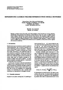
f (x; w). Clearly, placing a prior p(w|θ) induces a distribution over functions, where the type of functions supported depends on the relationship of w to the function value. For example, if one expects a linear input-output relationship to exist in the data then a good choice would be f (x; w) = w> x. The functions supported by the prior, and thus the posterior, will then only include functions linear in the input. A set of functions drawn from such a “linear function” prior is illustrated in Figure 1.1. 4 3 2 1
0 −1
−2 −3
−4 −1
−0.5
0
0.5
1
Figure 1.1: 50 functions over {−1, 1} drawn from the prior induced by w ∼ N (0, I2 ). Notice how the marginal standard deviation increases with distance from origin – this is a direct result of the prior supporting linear functions only. The greyscale highlights a distance of 2 standard deviations from 0.
Representing functions with a finite number of parameters allows function learning to take place via the learning of w: p(w|y, X, θ) = where Z(θ) = p(y|X, θ) =
p(y|w, X, θ)p(w|θ) , Z(θ)
(1.1)
Z
(1.2)
p(y|w, X, θ)p(w|θ)dw,
is the normalizing constant, also known as the marginal likelihood of the model specified by hyperparameters θ, because it computes precisely the likelihood of observing the given dataset given the modelling assumptions encapsulated in θ. As a result, it also offers the opportunity to perform model adaptation via optimization with
2
respect to θ. Of course, if the problem at hand requires averaging over models with different hyperparameters to improve predictions (e.g. if the dataset is small), it is possible to add another layer to the hierarchy of Bayesian inference. The posterior in Equation 1.1 can be used directly to compute both the expected value of the underlying function f (x? ; w) and its variance at input location x? , through evaluating µ? = Ep(w|y,X,θ) (f (x? ; w)) , � σ?2 = Ep(w|y,X,θ) f (x? ; w)2 − µ2? .
(1.3) (1.4)
Thus, we can predict the function value and, perhaps equally importantly, report how certain we are about our prediction at any input location, as is required for the task of regression. An example of Equations 1.1 through 1.4 in action is given by Bayesian linear regression, for which: • f (x; w) = w> x. • p(w|θ) = N (w; 0, Σ). • p(y|w, X, θ) =
QN
i=1
N (yi ; w> x, σn2 ).
The prior covariance Σ is usually a diagonal matrix with D independent parameters. The likelihood term p(y|w, X) encodes the assumption that the observations are the true function values corrupted with zero mean IID Gaussian noise with variance σn2 . The hyperparameters include the parameters in Σ and the noise variance. Because both the prior and the likelihood are Gaussian it follows that the posterior p(w|y, X, θ) is also Gaussian and Z(θ) can be calculated analytically: p(w|y, X, θ) = N (µN , ΣN ), � 1 log Z(θ) = − y> Σ−1 E y + log(det(ΣE )) + N log(2π) , 2
3
(1.5) (1.6)
where 1 ΣN X> y, σn2 � �−1 1 > −1 = Σ + 2X X , σn = XΣX> + σn2 IN .
µN =
(1.7)
ΣN
(1.8)
ΣE
(1.9)
The predictive distribution at x? also becomes a Gaussian and is fully specified by µ? and σ?2 µ? = µ> N x? ,
(1.10)
σ?2 = x? > ΣN x? .
(1.11)
For a list of standard Gaussian identities, see Appendix A. The posterior distribution over functions implied by Equation 1.5 given a synthetic dataset is shown in Figure 1.2. Note how the predictive mean in Equation 1.10 is linear in the training targets, and how the predictive variance in Equation 1.11 does not depend on the targets at all – these are hallmark properties of analytically tractable regression models. In addition, it can be seen from Equation 1.6 that Z(θ) is a complicated non-linear function of the hyperparameters, indicating that attempts to integrate them out will have to resort to approximate inference techniques such as MCMC (for a recent example, see Murray and Adams [2010]). Hyperparameter optimization is an easier and well-justified alternative as long as there is enough data. As shown in O’Hagan and Forster [1994] and Jaynes [2003], the hyperparameter posterior will tend to a Gaussian distribution (i.e., a unimodal one) in the infinite data limit, given certain conditions which are usually satisfied by the standard GP setup. Furthermore, asymptotic Gaussianity applies because: p(θ|y) ∝
N Y i=1
p(yi |θ, y1 , . . . yi−1 )p(θ),
4
(1.12)
and it is usually the case that N 1 X ∂ 2 log p(yi |θ, y1 , . . . yi−1 ) p → − k, as N → ∞, k 6= 0. N i=1 ∂θ2
(1.13)
The condition in Equation 1.13 can be interpreted as requiring that the observations do not get less and less “informative” about θ. Suppressing dependence on input locations and integrating out the latent function, Equation 1.12 can be viewed as describing the GP hyperparameter posterior, given that the likelihood terms correspond to the GP marginal likelihood evaluated using the chain rule of probability. For GP models, it is usually the case that every observation is informative about the hyperparameters, except in cases where, for example, we have coincident inputs. 1.5
1
0.5
0
−0.5
−1 −1
−0.5
0
0.5
1
Figure 1.2: The bold line shows the posterior mean, and the greyscale errorbars show 2 times the marginal posterior standard deviation, given the data (shown as magenta points). The coloured lines represent 5 samples from the posterior.
The flexibility of the linear regression model can be increased by mapping the inputs x into some possibly higher-dimensional feature space through some feature mapping φ, although linearity in the parameters w must be retained to ensure analytic tractability. Furthermore, the expressions for the posterior, marginal likelihood and predictive distributions remain mainly unchanged – all that is required is to replace every occurrence of an input location xi with its feature mapping φ(xi ) ≡ φi . If the underlying function f (x; w) is assumed to be nonlinear in w, then Equations 1.1 through 1.4 become analytically intractable and one must resort to approximate
5
inference methods.
Bayesian Nonparametric Regression While conceptually simple, the parametric way of placing a distribution over functions suffers from several shortcomings. Firstly, the parameters in w are simply coefficients, so it is difficult in practice to specify a prior over them which correctly captures our intuitive beliefs about functional characteristics such as smoothness and amplitude. For example, let’s imagine we are employing the linear model outlined above in some feature space. It is hard to map a prior over the coefficient of say a polynomial feature φ(x) = xai xbj xck for a, b, c ∈ Z+ to properties such as smoothness and differentiability. As a result, both the prior and the posterior over w can get difficult to interpret. Secondly, when attempting to model complex input-output relationships the number of parameters can get large. Of course, we avoid the risk of overfitting by integrating over the parameter vector, however, a large parameter vector can result an uncomfortably large number of hyperparameters. The hyperparameter vector may grow even further as a result of using hand-crafted features with their own internal parameters. Hence, overfitting can return to haunt us during hyperparameter optimization. It is natural to therefore ask whether there is an direct way of placing a prior over the underlying function f . The answer lies in the use of stochastic processes, which are distributions over functions, by definition 1 . For regression the simplest stochastic process which serves the purpose is the Gaussian process (GP). The method for describing a distribution over functions (which are infinite dimensional) is accomplished through specifying every finite dimensional marginal density implied by that distribution. Conceptually the distribution over the entire function exists “in the limit”. This leads us to the following definition of the GP: Definition 1. The probability distribution of f is a Gaussian process if any finite selection of input locations x1 , . . . , xN gives rise to a multivariate Gaussian density over the associated targets, i.e., p(f (x1 ), . . . , f (xN )) = N (mN , KN ), 1
(1.14)
Stochastic processes were originally conceived to be distributions over functions of time, however, it is possible to extend the idea to multidimensional input spaces.
6
where mN is the mean vector of length N and KN is the N -by-N covariance matrix. The mean and covariance of every finite marginal is computed using the mean function and the covariance function of the GP respectively. As is the case for the Gaussian distribution, the mean and covariance functions are sufficient to fully specify the GP. The mean function µ(x) gives the average value of the function at input x, and is often equal to zero everywhere because it usually is the case that, a priori, function values are equally likely to be positive or negative. The covariance function k(x, x0 ) ≡ Cov(f (x), f (x0 )) specifies the covariance between the function values at two input locations. For the prior over functions to be proper, the covariance function has to be a positive definite function satisfying the property that RR h(x)k(x, x0 )h(x0 )dxdx0 > 0 for any h except h(x) = 0. For any finite marginal of the GP as defined above we have that, for i, j = 1, . . . , N : mN (i) = µ(xi ),
(1.15)
KN (i, j) = k(xi , xj ).
(1.16)
This is a consequence of the marginalization property of the Gaussian distribution, namely that if: " #! " # " #! a µa Ka,a Ka,b p =N , , (1.17) b µb Kb,a Kb,b then the means and covariances of marginals are simply the relevant subvectors and submatrices of the joint mean and covariance respectively, i.e., p(a) = N (µa , Ka,a ) and p(b) = N (µb , Kb,b ). Indeed, this is exactly what is happening in Equations 1.15 and 1.16 – we are simply reading out the relevant subvector and submatrix of the infinitely long mean function and the infinitely large covariance function. Of course, we will never need access to such infinitely large objects in practice because we only need to query the GP at training and test inputs, which form a finite set. For a rigorous introduction to the theory of GPs, see Doob [1953]. The definition of a GP allows function learning to take place directly through distributions over function values and not through surrogate parameter vectors, namely p(y|f , X, θ)p(f |X, θ) , (1.18) p(f |y, X, θ) = Z(θ)
7
and Z(θ) = p(y|X, θ) =
Z
p(y|f , X, θ)p(f |X, θ)df .
(1.19)
Conditioning the GP prior over f on the input locations X restricts attention to the finite marginal of the GP evaluated at X. Therefore, p(f |X, θ) = N (mN , KN ), where θ now includes any parameters that control the mean and covariance function. In the following the mean function will always be assumed to equal the zero function, so we can further write p(f |X, θ) = N (0, KN ). Note also that the integral used to compute the marginal likelihood in Equation 1.19 reduces to an N -dimensional integral. We assume the same noise model for the targets as we did for the parametric linear regression model – they are the true function values corrupted by IID Gaussian noise. Thus, the likelihood is simply p(y|f , X, θ) = N (f , σn2 IN ). As we once again have a Gaussian prior with a Gaussian likelihood we can evaluate the expression in Equations 1.18 and 1.19 analytically: p(f |y, X, θ) = N (mN |y , KN |y ), � 1 log Z(θ) = − y> K−1 E y + log(det(KE )) + N log(2π) . 2
(1.20) (1.21)
The expressions for the posterior mean and covariance and that for the marginal likelihood are quite similar to their parametric counterparts: 1 KN |y y, σn2 � �−1 1 −1 = KN + 2 IN , σn = KN + σn2 IN .
mN |y =
(1.22)
KN |y
(1.23)
KE
(1.24)
Note that the posterior over f is also an N -dimensional Gaussian as it is also conditioned on the training inputs X. Given the posterior over the underlying function values, we can make predictions (1) (M ) at M test inputs X? ≡ [x? , . . . , x? ] jointly. So far the equations derived have all assumed M = 1, however, with GPs we can predict jointly almost as easily as predicting individual test points so our predictive equations will be slightly more general than usual. Let f ? be the random vector representing the function values at
8
X? . Then, p(f ? |X? , X, y, θ) =
Z
p(f ? |X? , X, f , θ)p(f |X, y, θ)df ,
(1.25)
where the term p(f ? |X? , X, f , θ) can be derived directly from the definition of a GP. Furthermore, since " #! f p =N f?
" # " #! 0 KN KN M , , 0 KM N KM
(1.26)
where KM N is the cross-covariance of the training and test inputs and KM the covariance of the latter, standard Gaussian conditioning (see Appendix A) shows that � −1 p(f ? |X? , X, f , θ) = N KM N K−1 f , K − K K K . (1.27) M M N N M N N
Equation 1.25 is once again an integral of a product of two Gaussian densities. Thus, the predictive density is a Gaussian: p(f ? |X? , X, y, θ) = N (µ? , Σ? ).
(1.28)
It can be shown, using identities in Appendix A, that µ? = KM N KN + σn2 IN
�−1
y,
Σ? = KM − KM N KN + σn2 IN
�−1
(1.29) KN M .
(1.30)
The marginal likelihood expression in Equation 1.21 and the predictive mean and covariances in Equations 1.29 and 1.30 are the bread and butter of Gaussian process regression and are summarized below:
9
Gaussian Process Regression Equations � 1 > y (KN + σn2 IN )−1 y + log(det((KN + σn2 IN ))) + N log(2π) . 2 �−1 = KM N KN + σn2 IN y. �−1 = KM − KM N KN + σn2 IN KN M .
log Z(θ) = − µ? Σ?
Covariance functions Although we have introduced GP regression for any valid covariance function1 , many of the results in this thesis will involve a couple of frequently used kernels. The common characteristic of the covariance functions used is that they are all functions of a (scaled) distance δ between inputs x and x0 , where δ 2 = (x − x0 )> Λ(x − x0 ),
(1.31)
where Λ is a diagonal matrix with Λ(d, d) ≡ 1/`2d for d = 1, . . . , D. Covariance functions which are a function of absolute distance between input locations are known as stationary, isotropic kernels because they are invariant to translating or rotating the observations in input space. The squared exponential covariance function2 is probably the most popular example because it gives rise to very smooth (infinitely mean-square differentiable) functions, and is defined as follows3 : 0
k(x, x ) ≡ k(δ) =
σf2
�
δ2 exp − 2
�
.
(1.32)
The Mat´ern(ν) family of covariance functions are used when control over differentiability is required. The functions generated by the Mat´ern kernel are k-times 1
Also referred to in the literature as a kernel in order to highlight the connection to frequentist kernel methods. 2 In order to remain consistent with the literature we will stick to the term “squared exponential”, while noting that a better name would be exponentiated quadratic. 3 If the covariance function is isotropic we will “overload” it in the text by sometimes referring to as a function of δ only.
10
mean-square differentiable if and only if ν > k. Expressions for the Mat´ern kernel for ν = 21 , 32 , 25 , 72 are given below (at half-integer values of ν, the expressions become considerably simpler): (1.33) kν=1/2 (x, x0 ) = σf2 exp(−δ), � √ � √ kν=3/2 (x, x0 ) = σf2 (1 + 3δ) exp − 3δ , (1.34) � � � √ � √ 1 √ (1.35) kν=5/2 (x, x0 ) = σf2 1 + 5δ + ( 5δ)2 exp − 5δ , 3 � � � √ � √ 2 √ 2 1 √ 3 0 2 kν=7/2 (x, x ) = σf 1 + 7δ + ( 7δ) + ( 7δ) exp − 7δ . (1.36) 5 15 The kernel in Equation 1.33 is also known as the exponential covariance function and gives rise to the Ornstein-Uhlenbeck process which is not mean-square differentiable yet mean-square continuous. It can be shown that in the limit where ν → ∞ the Mat´ern kernel converges to the squared-exponential. In practice, since it is hard to learn high frequency components from noisy observations, the performance of a prior supporting infinitely-differentiable functions will not be significantly different from one supporting up to, say, three-times differentiable functions. For formal definitions of mean-square differentiability and continuity refer to Papoulis et al. [2002]. Figure 1.3 shows samples of function values drawn from GP priors implied by the squared-exponential and Mat´ern kernels for different values of σf2 and `1 over a scalar input space. Clearly, [`1 , . . . , `D ] control the characteristic lengthscales of the function along each input dimension – i.e., how rapidly they wiggle in each direction. The parameter σf2 is simply a scaling of the covariance and thus controls the amplitude of the functions generated. Notice how, with D + 1 parameters, we have been able to capture most intuitive functional properties succinctly. This is a major advantage of GP regression. An example regression with synthetic data is shown for the squared-exponential covariance in Figure 1.4. Many standard regression models can be cast as a GP with a specific covariance function. This is because any regression model which implicitly assigns a Gaussian density to latent function values is by definition doing what a GP does. Looking back at the previous section one can easily see (e.g. from Equation 1.9) that the parametric linear model is assigning the Gaussian N (0, Φ> ΣΦ) to the functions values at the training inputs, where Φ ≡ [φ1 , . . . , φN ]. Thus this model is a GP
11
ℓ = 1. 0, σ f = 1
ℓ = 1. 0, σ f = 5
10
10
5
5
0
0
−5
−5
−10 −1
0
−10 −1
1
ℓ = 0. 1, σ f = 1 10
5
5
0
0
−5
−5
0
1
ℓ = 0. 1, σ f = 5
10
−10 −1
0
−10 −1
1
0
1
Figure 1.3: Functions drawn from squared-exponential (in black) and Mat´ern(3/2) (in blue) covariance functions for different hyperparameter values. Mat´ern(3/2) kernels give rise to “rougher” function draws as they are only once-differentiable.
with covariance function k(x, x0 ) = φ(x)> Σφ(x). Many more examples linking a variety of regression techniques (ranging from neural networks to splines) to GPs is given in Rasmussen and Williams [2006].
1.2
Generalised Gaussian Process Regression [..]
In the standard GP regression setting, it is assumed that the likelihood is a fullyfactorized Gaussian, i.e.: p(y|f , X, θ) =
N Y i=1
N (yi ; fi , σn2 ).
(1.37)
We will refer to the problem where the likelihood is fully-factorized but non-Gaussian as generalised GP regression, i.e.: p(y|f , X, θ) =
N Y i=1
p(yi |fi , η) | {z }
Non-Gaussian factor
12
.
(1.38)
1.4 1.2 1 0.8 0.6 0.4 0.2 0 −0.2 −0.4 −1
−0.5
0
0.5
1
Figure 1.4: An example GP regression with the squared-exponential kernel. The bold black line shows the marginal posterior means and their 95% confidence intervals are show in greyscale. The coloured lines represent 5 samples from the posterior.
This extension captures a very large number of modelling tasks. For example, in the case of binary classification, where the targets yi ∈ {−1, 1} one cannot use a Gaussian. Instead we would like to be able to use likelihoods such as: p(yi = 1|fi , η) = 1 − p(yi = −1|fi , η) =
1 , 1 + exp(−fi )
(1.39)
or p(yi = 1|fi , η) = Φ(yi fi ),
(1.40)
where Φ is the Gaussian CDF and η is empty. In a task where we would like to model count data, we may want a likelihood such as: p(yi |fi , η) = Poisson(exp(fi )),
(1.41)
and so on. Much as in the case for standard regression, we would like to be able to compute the following key quantities. The first is the posterior distribution of f at the training inputs: p(y|f )p(f |X, θ) p(f |y, X, θ) = , (1.42) p(y|X, θ)
13
where p(y|X, θ) is the marginal likelihood of the data, used for the purposes of model comparison to select suitable θ: p(y|X, θ) =
Z
p(y|f )p(f |X, θ)df .
(1.43)
In addition, we would like to have a predictive distribution at unseen input locations X? : Z p(y? |X, y, X? , θ) =
where p(f ? |X, y, X? , θ) =
Z
p(y? |f ? )p(f ? |X, y, X? , θ)df ? ,
(1.44)
p(f ? |f , X? , θ)p(f |y, X, θ)df .
(1.45)
It is sometimes deemed sufficient to compute ˆf ? ≡ E (f ? |X, y, X? , θ) ,
(1.46)
ˆ ≡ p(y? |ˆf ? ). For certain tasks, such as and the associated predictive probabilities p ˆ gives the same test error rate (i.e., binary classification, labelling test cases using p the proportion of cases mislabelled) as that computed using Equation 1.44, so we ˆ instead of the “correct” predictive probabilities given do not lose much by using p in Equation 1.44. Given the likelihood p(y|f ) is non-Gaussian, one has to resort to approximate inference techniques for the computation of all these quantities. The field of approximate inference is a very large one, ranging from MCMC to variational Bayes. Two of the most commonly used approximate inference techniques for generalised GP regression include Laplace’s Approximation, which we summarize below, and the Expectation Propagation (EP) algorithm due to Minka [2001], which is introduced in Chapter 2 in the context of efficient generalised Gauss-Markov processes. For a good reference on how to use both these techniques in the context of (unstructured) GP regression, see Rasmussen and Williams [2006]. For an in-depth comparison of the approximations provided by these two methods, see Nickisch and Rasmussen [2008]. We will apply both Laplace’s approximation and EP in the context of several structured GP models in Chapters 2 and 4. In this thesis, we will be focussing primarily on the generalised regression task involving binary classification, although
14
most of the techniques presented will be applicable in the general case.
Laplace’s Approximation In Laplace’s approximation, the non-Gaussian posterior in Equation 1.42 is approximated as follows: p(f |y, X, θ) u N (ˆf , Λ−1 ), (1.47) where ˆf ≡ arg maxf p(f |y, X, θ) and Λ ≡ −∇∇ log p(f |y, X, θ)|f =ˆf . Let’s define the following objective: Ω(f ) ≡ log p(y|f ) + log p(f |X, θ). (1.48) Clearly, ˆf can be found by applying Newton’s method to this objective. The central iteration of Newton’s method is: f
(k+1)
←f
(k)
�
− ∇∇Ω(f
(k)
�−1 ) ∇Ω(f (k) ).
(1.49)
Given KN is the training set covariance matrix, it is straightforward to show that: ∇Ω(f ) = ∇f log p(y|f ) − K−1 N f,
∇∇Ω(f ) = ∇∇f log p(y|f ) −K−1 N , | {z } ≡−W � �−1 � (k+1) (k) −1 (k) ∇ log p(y|f )| − K f . f ← f + K−1 + W (k) f N N f
(1.50) (1.51) (1.52)
Convergence is declared when there is a negligible difference between f (k+1) and f (k) . Newton’s method is guaranteed to converge to the global optimum, given the objective in Equation 1.48 represents a convex optimisation problem w.r.t. f . This is true for many cases of generalised GP regression, as the log-likelihood term is usually concave for many standard likelihood functions, and the prior term is Gaussian and therefore log-concave, giving a typical example of a convex optimisation problem, as illustrated in Boyd and Vandenberghe [2004]. Notice that we can use the second-order Taylor expansion of exp (Ω(f )) about ˆf to obtain the following approximation to the true marginal likelihood given in 1.43:
15
p(y|X, θ) =
Z
exp(Ω(f ))df � � Z 1 > ˆ ˆ ˆ u exp(Ω(f )) exp − (f − f ) Λ(f − f ) df . 2
(1.53) (1.54)
Thus, 1 N log p(y|X) u Ω(ˆf ) − log det Λ + log(2π). (1.55) 2 2 Also, note that since we have a Gaussian approximation to p(f |y, X, θ), the predictive distribution in Equation 1.45 can be computed using standard Gaussian identities, although further approximations may be required to compute the expression in Equation 1.44. For further details on these issues, see Rasmussen and Williams [2006].
1.3
The Computational Burden of GP Models
Gaussian Process Regression GPs achieve their generality and mathematical brevity by basing inference on an N -dimensional Gaussian over the latent function values f . Algorithm 1 gives the pseudo-code used for computing the marginal likelihood Z(θ) and the predictive density N (µ? , Σ? ), and shows that the computational cost of working with an N dimensional Gaussian is O(N 3 ) in execution time and O(N 2 ) in memory. The complexity of the Cholesky decomposition central to GP regression1 is quite severe for large datasets. For example, a dataset containing 20,000 observations (this is not even classed as large nowadays) will take hours to return. Of course, this is assuming that it runs at all – 20,000 observations will require roughly 7GB of memory, and many operating systems will refuse to run a program with such memory requirements! One can argue that the exponential increase in computing power will allow computational resources to catch up with the complexity inherent in GP models. However, typical dataset sizes in industry are also experiencing The Cholesky decomposition is the preferred way to compute K−1 y due to its numerical stability. 1
16
Algorithm 1: Gaussian Process Regression inputs : Training data {X, y}, Test locations X? , Covariance Function covfunc, hyperparameters θ = [σf2 ; `1 . . . `D ; σn2 ] outputs: Log-marginal likelihood log Z(θ), predictive mean µ? and covariance Σ? 1 2 3 4 5 6 7 8 9
KN ← covfunc(X,θ); //Evaluate covariance at training inputs 2 //Add noise KN ← KN + σn IN ; 3 L ← Cholesky(KN ); //O(N ) time, O(N 2 ) memory α ← Solve(L> , Solve(L, y)); //α = (KN + σn2 IN )−1 y [KM , KM N ] ← covfunc(X, X? , θ); V ← Solve(L, KM N ); µ? ← KM N α; > Σ? ← KM − V� V; � P N L(i, i) + log(2π) ; log Z(θ) ← − 21 y> α + N i=1 2
rapid growth as more and more aspects of the physical world are computerized and recorded. As a result, there is a strong incentive for applied machine learning research to develop techniques which scale in an acceptable way with dataset size N. A significant amount of research has gone into sparse approximations to the full GP regression problem. In the full GP, N function values located at the given input locations give rise to the dataset. Most sparse GP methods relax this by assuming that there are actually P latent function values, ¯f , located at “representative” input ¯ giving rise to the N input-output pairs, where P � N . The training locations1 , X, targets y are used to derive a posterior distribution over ¯f and this posterior is used to perform model selection and predictions. This has the effect of reducing run-time complexity to O(P 2 N ) and memory complexity to O(P N ), a noteworthy improvement. The pseudo-input locations are learned, manually selected or set to be some subset of the original input locations, depending on the algorithm. A good example of this type of method is given by the FITC approximation, see Snelson and Ghahramani [2006]. Other sparse GP techniques involve low-rank matrix approximations for solving the system (KN + σn2 IN )−1 y (e.g., see Williams and Seeger [2001]) and frequency domain (e.g., L´azaro-Gredilla [2010]) methods. For an excellent review of 1
also known as pseudo-inputs.
17
sparse GP approximations, see Qui˜ nonero-Candela and Rasmussen [2005]. The improved computational complexity of sparse GPs comes at the expense of modelling accuracy, and, at present, an increase in the number of failure modes. The former is inevitable: we are throwing away information, albeit intelligently. An example of the latter can be seen in the FITC algorithm. The need to select or ¯ runs the risk of pathologically interacting with the process of hyperparamlearn X eter learning and reviving the problem of overfitting as explained in Snelson and Ghahramani [2006]. A very clear advantage of these methods however is their generality – they work with any valid covariance function, and with an arbitrary set of inputs from RD .
Generalised Gaussian Process Regression The runtime complexity of generalised GP regression is O(N 3 ) although usually with a constant that is a multiple of the one for the standard regression task. The memory complexity is similar and O(N 2 ). Thus, unsurprisingly, generalised GP regression suffers from similar scaling limitations. For example, referring to Equation 1.52, we can see that each Newton iteration of Laplace’s approximation runs in O(N 3 ) time and O(N 2 ) space. A similar iterative scheme comes about as a result of applying EP – see Rasmussen and Williams [2006]. Despite suffering from higher computational demands, there is a much smaller number of techniques in the literature that deal with improving the complexity of generalised GP regression. It is fair to say that this is an active area of GP research. Current solutions can be characterized as attempts to combine the idea of sparse GP methods with approximate inference methods necessary to handle nonGaussian likelihoods. A good example is the Informative Vector Machine (IVM), which combines a greedy data subset selection strategy based on information theory and assumed density filtering (which is used to deal with non-Gaussianity) Lawrence et al. [2003]. Another example is the Generalised FITC approximation of Naish-Guzman and Holden [2007] which combines FITC with EP. Similar to their regression counterparts, these methods trade-off modelling accuracy with reduced complexity, although arguably they suffer from a larger array of failure modes. Furthermore, these methods do not assume any structure in the underlying covariance,
18
and thus are, in a sense, orthogonal to the approaches we will use in this thesis to improve efficiency in the generalised regression setting.
1.4
Structured Gaussian Processes
The central aim of this thesis is to demonstrate that there exist a variety of useful structured GP models which allow efficient and exact inference, or at the very least allow a superior accuracy/run-time trade-off than what is currently available for generic GP regression. We define what we mean by a structured GP as follows: Definition 2. A Gaussian process is structured if its marginals p(f |X, θ) contain exploitable structure that enables reduction in the computational complexity of performing regression. A somewhat trivial example is given by the GP with the linear regression covariance function introduced in the previous section, for which k(x, x0 ) = φ> Σφ and thus KN = Φ> ΣΦ. Let’s assume the size of Φ is F × N with F � N and that, as usual, Knoise is diagonal. We can then compute the troublesome quantities (KN + Knoise )−1 y, (KN + Knoise )−1 KN M and det(KN + Knoise ) in O(N F 2 ) time and O(N F ) memory by appealing to the matrix inversion lemma and the associated matrix determinant lemma: � −1 > > −1 (KN + Knoise )−1 = K−1 Σ−1 + ΦK−1 ΦK−1 noise − Knoise Φ noise Φ noise , (1.56) � > det(KN + Knoise ) = det Σ−1 + ΦK−1 det(Σ) det(Knoise ). (1.57) noise Φ
Clearly, exact inference can be performed for such a structured GP model much more efficiently. The reduction in complexity is clearly a result of the low-rank nature of the (noise-free) covariance function. In the special case where φ(x) = x the covariance function gives rise to covariance matrices of rank D. The improvement in computation comes as a direct consequence of the rather strong assumption that the input-output relationship is linear. In this thesis, we present a set of algorithms that make different types of assumptions, some of which turn out to be strong for certain datasets, and some which are perfectly suitable for a host of applications.
19
1.5
Outline
Over the course of the thesis we will make four different types of assumptions which turn out to have significant efficiency implications for standard and generalised GP regression. The first is where we consider Gaussian processes which are also Markovian. This assumption results in a computationally far more attractive factorization of the marginal p(f |X, θ), as demonstrated in Hartikainen and S¨arkk¨a [2010]. As GaussMarkov processes are strictly defined over “time” (or any scalar input space) we will initially restrict attention to regression on R (Chapter 2), although we will also explore GP models which allow the efficiency gains to be carried over to regression on RD in Chapter 4. We will show that, especially in 1D, the Markovian assumption is indeed a very weak one and that, as a result, we do not lose much in terms of generality. Despite this generality, the Markovian assumption allows us to construct exact (or near-exact) algorithms that have O(N log N ) runtime and O(N ) memory requirements, for both standard and generalised GP regression. Secondly, we attempt to introduce block structure into covariance matrices by means of assuming nonstationarity. Note that nonstationarity generally adds to the computational load, as is apparent in many case studies such as Adams and Stegle [2008] and Karklin and Lewicki [2005]. However, by limiting attention to a product partition model, as introduced in Barry and Hartigan [1992], we can exploit the nonstationary nature of the problem to improve complexity. Furthermore, a product partition model allows us to partition the input space into segments and fit independent GPs to each segment, in a manner similar to Gramacy [2005]. Dealing with nonstationarity can have the added benefit of actually producing predictions which are more accurate than the usual stationary GP, although approximations will be needed when working with the posterior over input space partitionings. We restrict attention to sequential time-series modelling in this thesis (Chapter 3), although, again, extensions as in Chapter 4 are applicable for nonstationary regression on RD . The assumption of nonstationarity is suitable to many real-world applications. In Chapter 4 we use the assumption of additivity to extend the efficiency gains obtained in Chapter 2 to input spaces with dimension D > 1. This assumption
20
would be suitable to cases where the underlying function values can be modelled well as a sum of D univariate functions. Somewhat unsurprisingly, inference and learning for a GP with an additive kernel can be decomposed into a sequence of scalar GP regression steps. As a result, with the added assumption that all additive components can be represented as Gauss-Markov processes, additive GP regression can also be performed in O(N log N ) time and O(N ) space. Similar efficiency gains can be also be obtained for Generalised GP regression with Laplace’s approximation. The assumption of additivity frequently turns out to be too strong an assumption for many large-scale real-world regression tasks. It is possible to relax this assumption by considering an additive model over a space linearly-related to the original input space. We will show that learning and inference for such a model can be performed by using projection pursuit GP regression, with no change to computational complexity whatsoever. Another interesting route to obtaining structured GPs involves making assumptions about input locations. It is a well-known fact that GP regression can be done in O(N 2 ) time1 and O(N ) memory when the inputs are uniformly spaced on R using Toeplitz matrix methods (see, e.g. Zhang et al. [2005] and Cunningham et al. [2008]). What has been unknown until now is that an analogue of this result exists for regression on RD for any D. In this case one assumes that the inputs lie on a multidimensional grid. Furthermore, the grid locations need not be uniformly spaced as in the 1D case. We demonstrate how to do exact inference in O(N ) time and O(N ) space for any tensor product kernel (most commonly-used kernels are of this form). This result is proved and demonstrated in Chapter 5. We conclude the thesis in Chapter 6 by discussing some interesting extensions one could follow up to build more GP implementations which scale well.
1
More involved O(N log N ) algorithms also exist!
21
Chapter 2 Gauss-Markov Processes for Scalar Inputs In this chapter, we firstly aim to drive home the message that Gauss-Markov processes on R can often be expressed in a way which allows the construction of highly efficient algorithms for regression and hyperparameter learning. Note that most the ideas we present for efficient Gauss-Markov process regression are not new and can be found in, e.g., Kalman [1960], Bar-Shalom et al. [2001], Grewal and Andrews [2001], Hartikainen and S¨arkk¨a [2010], Wecker and Ansley [1983]. Due in part to the separation between systems and control theory research and machine learning, the SDE viewpoint of GPs has not been exploited in commonly used GP software packages, such as Rasmussen and Nickisch [2010]. We are thus motivated to provide a concise and unified presentation of these ideas in order to bridge this gap. Once this is achieved, we contribute an extension that handles non-Gaussian likelihoods using EP. The result is a scalar GP classification algorithm which runs in O(N log N ) runtime and O(N ) space. For appropriate kernels, this algorithm returns exactly the same predictions and marginal likelihood as the standard GP classifier (which also uses EP).
2.1
Introduction
The goal of this chapter is to demonstrate that many GP priors commonly employed over R can be used to perform (generalised) regression with efficiency orders of
22
magnitude superior to that of standard GP algorithms. Furthermore, we will derive algorithms which scale as O(N log N ) in runtime and O(N ) in memory usage. Such gains come about due to the exact (or close to exact) correspondence between the function prior implied by a GP with some covariance function k(·, ·), and the prior implied by an order-m linear, stationary stochastic differential equation (SDE), given by: dm f (x) dm−1 f (x) df (x) + a0 f (x) = w(x), (2.1) + a + · · · + a1 m−1 m m−1 dx dx dx where w(x) is a white-noise process with mean 0 and covariance function kw (xi , xj ) = qδ(xi −xj ). Since white-noise is clearly stationary, we will also refer to its covariance function as a function of τ ≡ xi −xj , i.e., k(τ ) = qδ(τ ). q is the variance of the whitenoise process driving the SDE. Note that x can be any scalar input, including time. Because w(x) is a stochastic process, the above SDE will have a solution which is also a stochastic process, and because the SDE is linear in its coefficients, the solution will take the form of a Gaussian process. This is not an obvious result and we will expand on it further in Section 2.3. Furthermore, the solution function f (x) will be distributed according to a GP with a covariance function which depends on the coefficients of the SDE. We can rewrite Equation 2.1 as a vector Markov process: dz(x) = Az(x) + Lw(x), dx i> h df (x) dm−1 f (x) where z(x) = f (x), dx , . . . , dxm−1 , L = [0, 0, . . . , 1]> 1 , and
0 1 . . .. .. A= 0 0 −a0 · · ·
···
··· ··· ···
0 .. .
0 .. .
1 0 −am−2 −am−1
.
(2.2)
(2.3)
Equation 2.2 is significant because it dictates that given knowledge of f (x) and its m derivatives at input location x, we can throw away all information at any other input location which is smaller than x. This means that by jointly sorting 1
Note that in the exposition of the state-space representation of a GP, we will use capital letters for some vectors in order to remain consistent with the SDE literature. The motivation behind this stems from the fact that in a more general state-space model these objects can be matrices.
23
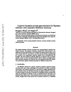
our training and test sets and by augmenting our latent-space to include derivatives of the underlying function in addition to the function value itself, we can induce Markovian structure on the graph underlying GP inference. All efficiency gains demonstrated in this chapter will arise as a result of the Markov structure inherent in Equation 2.2. In fact, the efficiency gains are so significant that the asymptotic runtime cost is dominated by the operation of sorting the training and test inputs! Figure 2.1 illustrates the reformulation of GP regression into a Markovian state-space model (SSM). In order to construct the SSM corresponding to a particular covariance function, it is necessary to derive the implied SDE. In Section 2.2 we illustrate the SDEs corresponding to several commonly used covariance functions including all kernels from the Mat´ern family and spline kernels, and good approximate SDEs corresponding to the squared-exponential covariance function. Once the SDE is known, we can solve the vector differential equation in Equation 2.2 and therefore compute the time and measurement update equations that specify all the necessary conditional distributions required by the graph in Figure 2.1. The Kalman filtering and RauchTung-Striebel (RTS) smoothing algorithms, which correspond to performing belief propagation on the graph using forward filtering and backward smoothing sweeps, can then be used to perform GP regression efficiently, see Kalman [1960] and Rauch et al. [1965]. Because we are dealing with Gaussian processes, all the conditional distributions involved are Gaussian. We will present the details on how to compute these given a GP prior in the form of an SDE in Section 2.3.
2.2
Translating Covariance Functions to SDEs
In Chapter 1 we described the GP prior in terms of its covariance function (and assumed its mean function be to be zero). In this Chapter, we would like to view the same prior from the perspective of Equation 2.1. In order to analyze whether or not it is possible to write down a SDE for a given covariance function and, if so, how to derive it, requires that we understand how to go in the opposite direction. In other words, given an SDE as in Equation 2.1, what is the implied covariance function of f (x) given that the covariance function of w(x) is kw (τ ) = qδ(τ )? The first step is to view the SDE as representing a linear, time-invariant (LTI)
24
x˜1
x˜2
x˜N
x˜�
...
...
f(·) : y˜1
y˜2
y˜N
y˜�
Sort dataset & augment state space
x1
xN
x�
...
...
z(·) :
y1
y�
yN
Figure 2.1: Illustrating the Transformation of GP Regression into Inference on a vector Markov process using Graphical Models. Unshaded nodes indicate latent variables, shaded ones are observed variables and solid black dots are variables treated as known in advance. In standard GP regression (illustrated in the top half) the hidden state variables are the underlying function values. They are fully connected as illustrated by the bold line connecting them. By augmenting the latent state variables to include m derivatives, we derive a chain-structured graph (illustrated in the bottom half). Reduction from a fully connected graph to one where the maximal clique size is 2 results in large computational savings. x and y are x ˜ and y ˜ sorted in ascending order. We see that in this example that the test point is the second smallest input location in the whole dataset.
system, driven by white-noise, as shown in Figure 2.2. For a good introduction to LTI systems, refer to Oppenheim et al. [1996]. Conceptually, for every sample of white-noise with variance q, the LTI system produces a sample from a GP with
25
LTI system : f (x) = T {w(x)} w(x)
L
�
+
z(x)
H
f (x)
A
Figure 2.2: The LTI system equivalent to the SDE in Equation 2.2. The components represent the vectors L and H and the matrix A in Equation 2.2. Conceptually, the “integrator” integrates the system in Equation 2.2 over an infinitesimal interval.
some covariance function. In order to determine what this covariance function is, it is necessary to characterize the output produced for an arbitrary, deterministic input function, φ(x). Because the internals of the black-box producing f (x) from w(x) are a sequence of linear operations, it is clear from this figure that, under appropriate initial conP P ditions, T { i αi φi (x)} = i αi T {φi (x)} for any αi and any input function φi (x). As T does not change as function of x, “time-invariance” is also satisfied. Every LTI system is fully characterized by its impulse response function, which is the output of the system when we input a unit impulse at time 0, i.e.: h(t) = T {δ(t)} .
(2.4)
The reason we can fully characterize an LTI system using h(t) is a consequence of the following theorem: Theorem 2.1. For any deterministic input φ(x), T {φ(x)} = φ(x) ? h(x). Proof. Since we can trivially write φ(x) = have
26
R∞
−∞
(2.5)
φ(x − α)δ(α)dα for any φ(x), we
�Z
�
∞
T {φ(x)} = T φ(x − α)δ(α)dα , −∞ Z ∞ = φ(x − α)T {δ(α)} dα, −∞ Z ∞ φ(x − α)h(α)dα, =
[linearity] [time-invariance]
−∞
≡ φ(x) ? h(x).
Taking the Fourier transform of both sides Equation 2.5 and using the convolution property, we can write: F (T {φ(x)}) ≡ F (ω) = Φ(ω)H(ω),
(2.6)
where Φ(ω) is Fourier transform of the (arbitrary) input, F (ω) that of the output and H(ω) that of the impulse response function, which is commonly known as the frequency response function. Using Theorem 2.1 it is straightforward to prove the following: Theorem 2.2. The covariance function of the output of an LTI system driven with a stochastic process with kernel kw (τ ) is given by: kf (τ ) = kw (τ ) ? h(τ ) ? h(−τ ).
(2.7)
Proof. Given that the system is linear and the mean function of the white-noise process is 0, it is clear that the mean function of the output process is also zero. Hence, kf (τ ) ≡ E (f (x)f (x + τ )) , ��Z ∞ � � =E w(x − α)h(α)dα f (x + τ ) , −∞ Z ∞ = E (w(x − α)f (x + τ )) h(α)dα, −∞
27
[2.1]
Z
∞
�
Z
�
∞
E w(x − α) w(x + τ − β)h(β)dβ h(α)dα, −∞ Z ∞ E (w(x − α)w(x + τ − β)) h(β)h(α)dβdα, = −∞ −∞ Z ∞Z ∞ kw (τ − β − γ)h(β)h(−γ)dβdγ, ≡ =
Z−∞ ∞
−∞
−∞
[2.1]
[γ ≡ −α]
≡ kw (τ ) ? h(τ ) ? h(−τ ).
Taking the Fourier transform of both sides of Equation 2.7 we can write:
Sf (ω) = Sw (ω)H(ω)H ∗ (ω),
(2.8)
= Sw (ω)|H(ω)|2 .
(2.9)
where Sw (ω) and Sf (ω) are the respective Fourier transforms of kw (τ ) and kf (τ ), also known as the spectral density functions of the input and output processes. Since, for a white-noise process, Sw (ω) = q 1 , the spectral density of the output GP becomes: Sf (ω) = qH(ω)H ∗ (ω) = q|H(ω)|2 .
(2.10)
For linear, constant coefficient SDEs we can derive H(ω) analytically by taking the Fourier transform of both sides of Equation 2.1. m X
dk f (x) ak = w(x). dxk k=0
m X
m
ak (iω)k F (ω) = W (ω).
k=0
Using Equation 2.6 we see directly that: F (ω) H(ω) = = W (ω)
m X k=0
ak (iω)k
!−1
.
(2.11)
Combining Equations 2.10 and 2.11 we see that if the spectral density of our GP 1
As the name implies!
28
can be written in the form Sf (ω) =
q . polynomial in ω 2
(2.12)
then we can immediately write down the corresponding SDE and perform all necessary computations in O(N log N ) runtime and O(N ) memory using the techniques described in Section 2.3.
2.2.1
The Mat´ ern Family
The covariance function for the Mat´ern family (indexed by ν) for scalar inputs is given by: 21−ν kν (τ ) = σf2 (λτ )ν Bν (λτ ) , (2.13) Γ(ν) where Bν is the modified Bessel function (see Abramowitz and Stegun [1964]) and √ we have defined λ ≡ `2ν . We had already seen examples of this family in Equations 1.33 through to 1.36. Recall that ` is the characteristic lengthscale and σf2 the signal variance. The Fourier transform of this expression and thus the associated spectral density is (see Rasmussen and Williams [2006]): S(ω) = σf2
q 2π 1/2 Γ(ν + 1/2)λ2ν ⇔ . 2 2 ν+1/2 Γ(ν)(λ + ω ) polynomial in ω 2
(2.14)
The spectral density of the Mat´ern kernel is precisely of the form required to allow an SDE representation. All we have to do is to find the frequency response H(ω) giving rise to this spectral density and then use Equation 2.11 to find the coefficients ak . Note that Equation 2.14 implies that q = σf2
2π 1/2 Γ(ν + 1/2)λ2ν . Γ(ν)
Using Equation 2.10 and 2.14 we can write:
29
(2.15)
S(ω) , q = (λ2 + ω 2 )−(ν+1/2) ,
H(ω)H ∗ (ω) =
= (λ + iω)−(ν+1/2) (λ − iω)−(ν+1/2) . Thus, H(ω) = (λ + iω)−(ν+1/2) .
(2.16)
For example, when ν = 7/2, the resulting SDE is given, in vector form, as follows:
0 1 0 0 0 0 0 1 0 dz(x) z(x) + 0 w(x). = 0 dx 0 0 1 0 4 3 2 −λ −4λ −6λ −4λ 1
(2.17)
where the variance of w(x) is q given by Equation 2.15. Note that the Mat´ern kernel is well-defined for ν ∈ R+ , although it may not be possible to derive an analytic expression for its corresponding SDE for non-halfinteger values of ν.
2.2.2
Approximating the Squared-Exponential Covariance
The squared-exponential is a kernel which is frequently used in practice, due in part to its intuitive analytic form and parameterisation. For completeness, we present ways in which one could approximate this covariance with an SDE, while noting that its support for infinitely differentiable functions makes it computationally rather unattractive. The Fourier transform of a squared-exponential kernel is itself a squared-exponential of ω, i.e.: k(τ ) =
σf2
�
τ2 exp − 2 2`
�
⇔ S(ω) =
√
2πσf2 ` exp
� � ω 2 `2 − . 2
(2.18)
We can write the spectral density in a form similar to Equation 2.12 using the Taylor
30
expansion of exp(x). S(ω) = �
√ 1+
ω 2 `2 2
+
2πσf2 ` 1 2!
� ω 2 `2 2 2
+ ...
�.
(2.19)
As the denominator is an infinitely long polynomial we cannot form an SDE which exactly corresponds to the SE kernel. This should come as no surprise since the SE covariance gives rise to infinitely differentiable functions. Therefore, conceptually, we would need to know an infinite number of derivatives to induce Markov structure. However, we can obtain an approximation by simply truncating the Taylor expansion at some maximum order M . By doing so, the approximate spectral density becomes a special case of Equation 2.12, and we can proceed to compute the frequency response function:
H(ω)H ∗ (ω) = =
S(ω) , q 1 ω 2 `2 + 1+ 2 2!
�
ω 2 `2 2
�2
1 + ··· + M!
�
ω 2 `2 2
�M !
.
H(ω) is thus a polynomial of iω, however, unlike the case for the Mat´ern kernel, we cannot find the coefficients of this polynomial analytically and will therefore have to resort to numerical methods (for further details, see Hartikainen and S¨arkk¨a [2010]). Alternatively, one may choose to assume that a member of the Mat´ern family with high enough ν (e.g. ν ≥ 7/2) is an acceptable approximation. This has the advantage of avoiding numerical routines for computing the SDE coefficients, at the expense of a small loss in approximation quality. Figure 2.3 illustrates the two alternatives for approximating the squared-exponential covariance.
2.2.3
Splines
Splines are regression models which are popular in the numerical analysis and frequentist statistics literatures (for a good introduction see Hastie et al. [2009]). Following Wahba [1990] and Rasmussen and Williams [2006], a connection can be made between splines of arbitrary order m and GPs. The frequentist smoothing problem
31
Matern:ν=1/2 [red] → SE [black]
Taylor Exp.: M=1 [red] → SE [black] 3
2.5
2.5
2
2 S(ω)
S(ω)
3
1.5
1.5
1
1
0.5
0.5
0
−2
0 ω
0
2
−2
0 ω
2
Figure 2.3: (Left) Spectral density of the Mat´ern kernels (with unit lengthscale and amplitude) for ν = [1/2, 3/2, . . . , 11/2] in shades of red; true squared-exponential spectral density in black. (Right) Spectral density of the Taylor approximations (with unit lengthscale and amplitude) for M = [1, . . . , 6] in shades of red; true squared-exponential spectral density in black. For a given order of approximation the Taylor expansion is better, however, we cannot find coefficients analytically.
is to minimize the cost-functional Ω(f (·)) ≡
N X i=1
2
(f (xi ) − yi ) + λ
Z
b
(f (m) (x))2 dx.
(2.20)
a
where λ is a regularization parameter (usually fit using cross-validation) which controls the trade-off between how well the function fits the targets (first term) and how wiggly/complex it is (second term). The minimization is over all possible functions f (x) living in a Sobolev space of the interval [a, b]. For an excellent introduction on functional analysis see Kreyszig [1989]. Interestingly, one can obtain a unique global minimizer which can be written as a natural spline: a piecewise polynomial of order 2m − 1 in each interval [xi , xi−1 ] and a polynomial of order m − 1 in the intervals [a, x1 ] and [xN , b]. A spline is generally not defined over all of R but over a finite interval from a to b, where a < min(x1 , . . . , xN ) and b > max(x1 , . . . , xN ). Therefore, without loss of generality, we can assume a = 0 and b = 1, requiring that
32
inputs be scaled to lie between 0 and 1. The natural spline solution is given by:
f (x) =
m−1 X j=0
β j xj +
N X i=1
γi (x − xi )2m−1 , where (z)+ ≡ +
z
if z > 0,
0 otherwise.
(2.21)
The parameters β ≡ {βj } and γ ≡ {γi } can be determined in O(N log N ) time and O(N ) space due to the Reinsch algorithm described in Green and Silverman [1994] and Reinsch [1967]. This algorithm also requires the sorting of inputs and the attains its efficiency by re-expressing the optimization as a linear system which is band-diagonal (with a band of width 2m + 1). The representer theorem Kimeldorf and Wahba [1971] indicates that the solution can be written in the following form: f (x) =
m−1 X
j
βj x +
j=0
N X
αi R(x, xi ),
(2.22)
i=1
where R(x, x0 ) is a positive definite function, as shown in Seeger [1999]. Both the nature of the solution and the complexity of attaining it have analogues in an equivalent GP (Bayesian) construction. The key to obtaining an efficient algorithm again lies in the SDE representation of GP priors, although in this case it won’t be possible to represent the SDE as an LTI system due to the nonstationarity of the spline kernel (see below). Let’s consider the following generative model representing our prior:
β ∼ N (0, B),
(2.23)
fsp (x) ∼ GP(0, ksp (x, x0 )), m−1 X f (x) = βj xj + fsp (x),
(2.24) (2.25)
j=0
yi = f (xi ) + �, where � ∼ N (0, σn2 ).
(2.26)
This setup is different from the standard GP prior introduced in Chapter 1 for two reasons. First, all inputs are assumed to be between 0 and 1. Secondly, it is a combination of a parametric model with a polynomial feature mapping φ(x) = [1, x, . . . , xm−1 ] and a separate GP prior which is effectively modelling the residuals
33
of the parametric component. In fact, it is an instance of an additive model (see Chapter 4). Due to the additive nature of the prior and the fact that we can represent the parametric component as a GP (as in Chapter 1), it is clear that the function prior implied by Equation 2.25 also gives rise to a GP. Its covariance function is given by the sum of the covariance functions of the two components, namely: kf (x, x0 ) = ksp (x, x0 ) + φ(x)> Bφ(x).
(2.27)
Note that we haven’t yet specified ksp (x, x0 ). We would like to set it so that after observing a dataset of size of N our maximum-a-posteriori (MAP) function estimate is in line with the frequentist solution presented in Equation 2.22. For GPs the MAP estimate is given by the posterior mean function, which we derived in Equation 1.29: µ(x) = k(x)> KN + σn2 IN
�−1
y,
(2.28)
where k(x) is the KM N matrix evaluated at the singleton test location, x, and KN is the training covariance matrix associated with the kernel in Equation 2.27. After some rearrangement, we can rewrite Equation 2.28 in a form consistent with Equation 2.22 � � ˆ + k> (x) K ˆ , ˜ −1 y − Φ> β (2.29) µ(x) = φ(x)> β sp sp {z } | ˆ ≡α
where ksp (x) is the cross-covariance vector associated with the kernel ksp (x, x0 ), ˆ is ˜ sp ≡ Ksp + σ 2 IN and Φ is the feature mapping applied to all training inputs. β K n the posterior mean of the parameters of the linear component of the model and is given by: � �−1 ˆ = B−1 + ΦK ˜ −1 y. ˜ −1 Φ> β ΦK (2.30) sp
sp
Because the coefficients β are assumed to be arbitrary in the frequentist setup, we would like to consider the limit where B−1 → 0, thus obtaining the posterior over β given an improper prior: � �−1 ˆ = ΦK ˜ −1 Φ> ˜ −1 y. β ΦK sp sp
(2.31)
Equation 2.29 makes intuitive sense since it states that the mean prediction at x is
34
the sum of the mean prediction of the linear component and the mean prediction of ˆ a GP which models the residuals y − Φ> β. Wahba [1990] showed that the mean function in Equation 2.29 is in line with the solution implied by the representer theorem if and only if we set ksp (·, ·) as the covariance function of the (m − 1)-fold-integrated Wiener process of amplitude σf2 1 . From a computational perspective this is great news because the (m − 1)-foldintegrated Wiener process is the solution to the following SDE: dm f (x) = w(x). dxm
(2.32)
For example, a quintic spline prior gives rise to the following vector-Markov process: 0 1 0 0 dz(x) = 0 0 1 z(x) + 0 w(x), dx 0 0 0 1
(2.33)
where the variance of w(x) is q ≡ σf2 . It is thus possible to compute the expressions in Equations 2.29 and 2.31 in O(N log N ) time and O(N ) space, using the techniques described in the following section. Additionally, given our Bayesian approach, we can compute the uncertainty in our regression estimate, using the standard equations in Chapter 1, at close to no additional computational cost. The predictive variance at test location x? can be written as follows: � � −1 −1 > > ˜ ˜ ρ, σ 2 (x? ) = ksp (x? , x? ) − k> (x ) K k (x ) + ρ Φ K Φ sp ? sp sp ? sp
(2.34)
where ˜ −1 ksp (x? ). ρ = φ(x? ) − ΦK sp 1
These are fundamental nonstationary stochastic processes.
35
(2.35)
2.3 2.3.1
GP Inference using State-Space Models The State-Space Model
In the previous section we showed how many different GP priors can be written as a vector Markov process, with state dynamics described by the equation: dz(x) = Az(x) + Lw(x). dx
(2.36)
Strictly, Equation 2.36 should be written in its integral form: √ dz(x) = Az(x)dx + L qdβ(x),
(2.37)
where dβ(x) ≡ w(x)dx is the infinitesimal increment of standard Brownian motion β(x) (also known as the Weiner process). For our purposes, Equation 2.37 is equivalent to 2.36 because we are only interested in integrating the SDE forward in time. Let’s assume that z(x) is Gaussian distributed with z(x) ∼ N (µ(x), Σ(x)). Taking the expectation of both sides of Equation 2.37 we can derive the ordinary linear differential equation describing the evolution of the mean:
dµ(x)= Aµ(x)dx, dµ(x) = Aµ(x), ⇒ dx
(2.38)
where we have used the fact that E(dβ(x)) = 0. Similarly, we can derive the evolution of the covariance matrix by considering the covariance of both sides of Equation 2.37.
⇒
� � dΣ(x)= AΣ(x) + (AΣ(x))> dx + qLL> dx dΣ(x) = AΣ(x) + Σ(x)A> + qLL> dx
(2.39)
where we have used Cov(dβ(x)) = Im dx and the fact that the Brownian motion is independent of z(x). This matrix differential equation is commonly referred to as the matrix Riccati differential equation (see, e.g., Willems [1971]). We can now use
36
Equations 2.38 and 2.39 to derive analytic expressions for µ(x) and Σ(x) given the initial conditions µ(x0 ) = µ0 and Σ(x0 ) = 0 (i.e., at x0 the process is deterministic). Furthermore, using the standard results in Riley et al. [2006] and Arnold [1992] we have: µ(x) = exp(A(x − x0 ))µ0 , (2.40) where we have used a matrix exponential. The matrix exponential is the exponential function generalized to square matrix arguments. Formally it is defined as follows: exp(X) =
∞ X 1 k X , k! k=0
(2.41)
where Xk is the matrix X matrix-multiplied with itself k times. For the covariance, we have the following unique and non-negative definite solution: Σ(x) = q
Z
x
x0
exp(−A(x − s))LL> exp(−A(x − s))ds,
(2.42)
where we have used the identity (exp(X))−1 = exp(−X). The integral in this Equation is over a matrix and is defined as the element-wise integral of its argument. Given the deterministic starting condition (which we have limited ourselves to) the density of z(x) is Gaussian for all x, and therefore µ(x) and Σ(x) capture all the uncertainty about z(x). See Arnold [1992] for a proof of this. Thus, all the conditional distributions in Figure 2.1 are Gaussians for the GP regression task and are listed below:
Initial state :
= N (z(x1 ); µ, V).
p(z(x1 ))
State update : p(z(xi )|z(xi−1 ))= N (z(xi ); Φi−1 z(xi−1 ), Qi−1 ). Emission : p(y(xi )|z(xi )) = N (y(xi ); Hz(xi ), σn2 ).
(2.43) (2.44) (2.45)
where we assume that the inputs xi are sorted in ascending order and may include test inputs, in which case we simply do not consider the emission distribution at that location. Using the above, we can write:
37
Φi−1 = exp(Aδi ), Z δi Qi−1 = q ci−1 (δi − h)c> i−1 (δi − h)dh,
(2.46) (2.47)
0
where δi ≡ xi − xi−1 and ci−1 is the last column of the matrix exp(A(δi − h)). The form of the emission distribution is very simple. H simply picks out the first element of the vector z(xi ) which corresponds to the latent function value inferred at location xi . In the case of the Mat´ern family and spline kernels, where we have obtained an analytic expression for A, it is also possible to derive an analytic expression for exp(At) using the following identity: � exp(At) = L−1 (sIM − A)−1 ,
(2.48)
where L−1 denotes the inverse Laplace transform and s ∈ C is a complex number. Equation 2.48 can be derived straightforwardly using properties of the Laplace transform. As a result, we can compute both the expressions in Equation 2.46 and 2.47 in closed form. For example, for the Mat´ern(3/2) kernel we obtain: Φi−1
" # (λδi + 1) δi 1 . = exp (λδi ) −(λ2 δi ) (1 − λδi )
(2.49)
Note that closed form expressions can be obtained for any Mat´ern order using a symbolic math package such as MATLAB’s Symbolic Math Toolbox (see Appendix B for code to generate these expressions automatically). Furthermore, when analytic expressions exist, the Symbolic Math Toolbox can also be used to to compute the integrals involved in computing Qi−1 (see Equation 2.47). In fact, there is a neat trick called matrix fraction decomposition which obviates the use of integrals for computing covariance matrices, as shown in S¨arkk¨a [2006]. Let’s return to the matrix Riccati differential equation in Equation 2.39. Assuming Σ(x) can be written as: Σ(x) = C(x)D(x)−1 ,
38
(2.50)
then by simply plugging in Equation 2.50 into both sides of the differential equation in 2.39, it can be seen that: dC(x) = AC(x) + qLL> D(x), dx dD(x) = −A> D(x). dx
(2.51) (2.52)
Amazingly, these system of equations can be expressed as one larger linear ODE, which in turn can be solved using matrix exponentials only: "
dC(x) dx dD(x) dx
#
"
A qLL> = 0 −A>
#"
# C(x) . D(x)
(2.53)
For a spline kernel of order m we can derive analytic expression for both the Φi−1 and the Qi−1 . Using Equations 2.46 and 2.47 we obtain: δim−1 δ2 1 δi 2!i . . . (m−1)! δim−2 0 1 δ . . . i (m−2)! , (2.54) Φi−1 = .. . . . . . . . . . . . . . 0 0 0 ... 1 Z δi (δi − h)m−j (δi − h)m−k Qi−1 (j, k) = q dh (2.55) (m − j)! (m − k)! 0 (m−j)+(m−k)+1
=
qδi . ((m − j) + (m − k) + 1)(m − j)!(m − k)!
(2.56)
These expressions are consistent with those derived in Wecker and Ansley [1983], who do not use the SDE representation of splines explicitly. If we do not have an analytic expression for A, as was the case for the Taylorexpansion based technique for approximating the squared-exponential kernel, then it is necessary to compute Φi−1 and Qi−1 numerically. As the coefficients in A are also found numerically (by solving polynomial equations), there is a tendency for numerical errors to propagate (causing, for example, matrices to become nonpositive definite). Indeed, we find that, in practice, this is a major disadvantage of using the Taylor-expansion based approximation, and will therefore stick to using high-order Mat´ern kernels for this task. In addition, one should be be wary of the
39
fact that computing derivatives of hyperparameters analytically becomes impossible if Φi−1 and Qi−1 are computed numerically. For SDEs described by LTI systems, µ = 0, because the starting state of the SDE (at x = −∞) is assumed to be 0 and because it is generally the case that limt→∞ exp(At) = 0, a property which is easily verified for Equation 2.49. More generally, the stability of a linear system implies non-positivity of the eigenvalues of A, so for any stable linear system it must be that µ = 0. We can compute V by considering what the process covariance tends to after running for an infinite interval, i.e., Z ∞
c(h)c> (h)dh,
V=q
(2.57)
0
where c is the last column of the matrix exp (Ah). The integral in Equation 2.57 always converges for LTI systems with absolutely integrable impulse response, i.e., for which Z ∞ |h(τ )|dτ < ∞. (2.58) −∞
It can be shown that the Mat´ern family and approximations to the squared-exponential covariance all give rise to LTI systems which satisfy this property. Alternatively, it is also possible to obtain V by solving the matrix Riccati equation, as in Bar-Shalom et al. [2001]: dV = AV + VA> + LqL> = 0. (2.59) dx Recall that for the spline kernel we limited the evolution of the SDE between input locations 0 and 1. To remain consistent with the literature, it suffices to set µ = 0 and Z x1 V=q c(h)c> (h)dh. (2.60) 0
Intuitively, we are starting the integrated Wiener process at the origin at x = 0 and considering its dynamics until x = 1.
2.3.2
Inference and Learning [..]
Now that we have specified how to compute all the necessary conditionals forming the state-space model, GP regression becomes a special case of performing inference on the chain-structured graph in Figure 2.1. After sorting the inputs, this
40
can be done in O(N ) runtime and space using the filtering-smoothing algorithm, which corresponds to running the generic belief propagation algorithm on our chainstructured graph. We would like to compute p(zk |y, x, θ) for k = 1 . . . K, where K = N + M as we have jointly sorted our training and input locations to form the vector x. The inference procedure consists firstly of a “forward” filtering run where p(zk |y1 , . . . , yi(k) , x, θ) are computed from k = 1, . . . , K in a recursive manner. i(k) gives the index of the target corresponding to state k in the Markov chain. The recursion is commonly known as the Kalman filter Kalman [1960]. The key equations are given below: (f )
(f )
p(zk−1 |y1 , . . . , yi(k−1) , x, θ) = N (µk−1 , Vk−1 ), w “Time” update (f )
(f )
p(zk |y1 , . . . , yi(k−1) , x, θ) = N (Φk−1 µk−1 , Φk−1 Vk−1 Φ> + Qk−1 ), | {zk−1 } ≡Pk−1 w Measurement update (f )
(f )
p(zk |y1 , . . . , yi(k) , x, θ) = N (µk , Vk ),
(f )
(f )
where µk = Φk−1 µk−1 , and Vk i(k) = i(k − 1) + 1, we have (f )
= Pk−1 if i(k) = i(k − 1). In the case where
(f )
(f )
µk = Φk−1 µk−1 + Gk [yi(k) − HΦk−1 µk−1 ],
(2.61)
Vk = Pk−1 − Gk HPk−1 ,
(2.62)
(f )
where Gk is known as the Kalman gain matrix : Gk = Pk−1 H> H> Pk−1 H + σn2 (f )
(f )
�−1
.
(2.63)
The recursion is initialized with µ1 = µ and V1 = V. Once the filtering densities are known, a backward recursive procedure, commonly known as the RTS smoother, updates p(zk |y1 , . . . , yi(k) , x, θ) to p(zk |y, x, θ) ≡ N (µk , Vk ) for k = K, . . . , 1, as follows:
41
� � (f ) (f ) µk = µk + Lk µk+1 − Φk µk ,
(2.64)
(f )
Vk = Vk + Lk (Vk+1 − Pk ) L> k,
(2.65)
−1 where Lk ≡ Vk Φ> k Pk is known as the Lyapunov matrix. The recursion is initialized (f ) (f ) using µK = µK and VK = VK . Note that the predictive density p(f (xk )|y, x, θ) has mean and variance given by µk = µk (1) and σk2 = Vk (1, 1). Algorithm 2 gives the pseudo-code for performing GP regression using state-space models. Note that this algorithm has been presented in the case where we know the locations of the test points in advance. This may not be the case in practice. Fortunately, due to the Markovian structure of the state-space model, we can predict at any new test input using the posterior distributions over the latent states at neighbouring training inputs (and there can be at most 2 neighbours). Recall that in the standard GP regression algorithm, the hyperparameters were learned by maximizing the marginal likelihood p(y|x, θ). When we can represent the GP model in state-space form, it is possible to use the Expectation-Maximization (EM) algorithm Dempster et al. [1977] to maximize the marginal likelihood with respect to the hyperparameters. The purpose of the EM algorithm is to avoid the direct maximization of the marginal likelihood, since finding analytic expressions for this quantity and its derivatives is often too difficult (or, indeed, not possible). Instead, one iteratively alternates between computing the expected complete data log-likelihood (EC ) (E-step) and optimising it w.r.t. the hyperparameters (M-step). Both these steps are often analytically tractable, which explains the wide-spread use of the EM algorithm. EC is given by:
EC (θ) ≡ Ep(Z|y,x,θold ) (p(Z, y|x, θ)) ,
(2.66)
where Z ≡ {zk }K k=1 . Referring to the graph in Figure 2.1 we can see that p(Z, y|x, θ) = log p(z(x1 ), θ) +
K X
log p(z(xt )|z(xt−1 ), θ) +
t=2
K X
log p(y(xt )|z(xt )).
t=1
(2.67) As we can push the expectation in Equation in 2.66 to the individual summands in
42
Algorithm 2: Gaussian Process Regression using SSMs inputs : Jointly sorted training and test input locations x. Targets y associated with training inputs. State transition function stfunc that returns Φ and Q matrices. Hyperparameters θ outputs: Log-marginal likelihood log Z(θ). Predictive means µ? and > variances v? . E-step moments: E(zt z> t ), E(zt zt−1 ) 1 2 3 4 5 6 7 8 9 10 11 12 13 14 15 16 17 18
(f )
(f )
µ0 ← µ; V0 ← V; Z(θ) = 0; for t ← 1 to K do if t > 1 then [Φt−1 , Qt−1 ] ← stfunc(θ, x(t) − x(t − 1)); else [Φt−1 , Qt−1 ] ←stfunc(θ, ∞); //Prior process covariance (f ) > Pt−1 ← Φt−1 Vt−1 Φt−1 + Qt−1 ; if is train(t) then (f ) log Z(θ) ← log Z(θ)+ gausslik(y(i(t)), HΦt−1 µt−1 , HPt−1 H> + σn2 ); (f ) (f ) (f ) µt = Φt−1 µt−1 + Gt [y(i(t)) − HΦt−1 µt−1 ]; (f ) Vt = Pt−1 − Gt HPt−1 ; else (f ) (f ) (f ) µt ← Φt−1 µt−1 ; Vt ← Pt−1 ; end end (f ) (f ) µK ← µK ; VK ← VK ; µ? (K) ← HµK ; v? (K) ← HVK H> ; > E(zK z> K ) ← VK + µK µK ; E(zK z> K−1 ) ← (ID − GK H)ΦK−1 VK−1 ; for t ← K − 1 to 1 do −1 Lt ← V t Φ> ; t Pt � � (f )
19 20 21 22 23 24 25
(f )
µt ← µt + Lt µt+1 − Φt µt (f )
; µ? (t) ← Hµt ;
> Vt ← Vt + Lt (Vt+1 − Pt ) L> t ; v? (t) ← HVt H ; > E(zt z> t ) ← Vt + µt µt ; if t < K − 1 then � > (f ) > > E(zt z> L + L E(z z ) ← V ) − Φ V Lt ; t+1 t+1 t+1 t+1 t+1 t t−1 t end end
43
Equation 2.67, the expectations computed in Algorithm 2 are sufficient to compute EC , and constitute the E-step of the EM algorithm. In the M-step we maximize Equation 2.66 with respect to θ, and repeat the process until convergence, as shown in Algorithm 3. The minimization can be accomplished using any off-the-shelf function minimizer, such as the one found in Rasmussen and Nickisch [2010]. Algorithm 3: Learning the hyperparameters using EM inputs : Training data {x, y}. Initial hypers θinit . outputs: Learned hyperparameters θopt . 1 2 3 4 5 6
θold ← θinit ; while (Z(θold ) − Z(θopt )) > � do Compute E-step moments using Algorithm 2 for θold ; //E-step Use E-step moments to evaluate and minimize −EC (θ) w.r.t θ; //M-step θold ← θopt ; end
2.4
Generalised Gauss-Markov Process Regression
So far, we have focussed on the case where the state-space representation of the GP prior has a Gaussian emission density (Equation 2.45). For many practical applications this assumption would not be appropriate, be it because the targets are categorical (as in classification) or represent counts (as in Poisson regression) or simply because Gaussian errors cannot handle outliers (in which case a Student-t error model would be a better choice). All of these cases can be dealt with by replacing the Gaussian emission density with a suitable likelihood function for p(y(xi )|z(xi )). For example, for 2-class classification where y(xi ) ∈ {−1, 1} one can use a probit likelihood: p(y(xi )|z(xi )) = Φ((Hz(xi ))yi ), (2.68) where Φ(·) is the standard Gaussian CDF. Inference and learning with non-Gaussian emissions necessitates the use of approximations to the true posterior over the latentstate Markov chain in Figure 2.1. There exist many algorithms for performing such an approximation, including variational inference and sequential Monte Carlo methods (for a thorough introduction, see Doucet et al. [2001]). However, we will
44
focus on Expectation propagation (EP), due to its superior approximation qualities (see e.g. Nickisch and Rasmussen [2008]) for GPs with non-Gaussian likelihoods. Moreover, it is shown in Minka [2001] that EP performs well for tree-structured graphs (it basically boils down to a “projected” Gaussian belief propagation) and we have spent most of this Chapter converting the GP regression graph into a chain structure!
2.4.1
Expectation Propagation [..]
The EP algorithm falls under the general framework of approximating an analytically and/or computationally intractable posterior distribution p(Z|D, θ) with a “simpler” distribution q(Z|D, θ), where Z represents all latent variables, D is the observed data and θ is a set of fixed hyperparameters. q is usually simpler than p in two ways. First, it is deemed to belong to the exponential family (for analytic convenience), and second, it is assumed to have a simpler factorization than p (for computational reasons). In this section, we will first present the EP algorithm for an arbitrary factor graph representing p, and assume that q is a fully-factorized Gaussian distribution over Z. We will illustrate the ideas using the application of EP to the graph in Figure 2.1, which is presented as a factor graph in Figure 2.5. Generally, the exact posterior will be proportional to a product of factors: Y
p(Z|D, θ) ∝
φi (Zne(φi ) ),
(2.69)
i
where Zne(φi ) is the subset of latent variables which are neighbours of factor φi . Our aim is to approximate this posterior using a product of Gaussian factors, each of which is a neighbour to only a single latent variable zk , i.e.: q(Z|D, θ) ∝
Y Y i
φ˜ik (zk ).
(2.70)
k∈ne(φi )
Ideally we would like to be able minimize
KL
1 p(D|θ)
Y i
φi (Zne(φi ) )
1 Zapprox
45
Y Y i
k∈ne(φi )
φ˜ik (zk ) ,
(2.71)
by matching the first and second moments of the marginals over the zk of the right-hand-side to those of the left-hand-side. The approximation to the evidence p(D|θ), given by Zapprox , can then be computed by normalising the unnormalised product of Gaussians on the right-hand-side. However, this ideal KL minimisation is intractable because it requires performing marginalization over the true posterior. In EP, we instead iterate across the individual factors φi according to a pre-determined schedule 1 and minimize, at each iteration, the following: hQ
KL
j6=i
Q
i ˜old (zk ) φi (Zne(φ ) ) φ i k∈ne(φj ) jk Zi
1 Zapprox
Y Y i
k∈ne(φi )
, φ˜new ik (zk )
(2.72) where ne(·) returns the variable neighbours of one or more factor variables, and vice versa. In many applications of EP, minimizing the divergence in Equation 2.72 via the matching of first and second moments is a tractable operation. Furthermore, marginals over the variables that are not in the neighbourhood of φi are unchanged. For variables which are in the neighbourhood of φi we have the following update equation:
∀k ∈ ne(φi )
φ˜new ik (zk ) ∝
Z Y old proj φ˜jk (zk ) j∈ne(zk ) j6=i
φi (Zne(φi ) )
Z¬k
Y
Y
zm ∈Z¬k `∈ne(zm )
Y
φ˜old jk (zk )
(2.73)
φ˜old `m (zm ) dZ¬k
.
j∈ne(zk ) j6=i
where we have defined Z¬k to be the set of variables connected to factor φi , excluding zk . This update is illustrated in Figure 2.4. The proj [·] operator takes a non-Gaussian argument and projects it to a Gaussian so that first and second moments of the Gaussian match those of the argument. If the argument turns out to be Gaussian then proj [·] is the identity. The proj [·] operator also computes the zeroth moment of its argument (since it is usually unnormalized) 1
In practice, the performance of EP is, unsurprisingly, sensitive to the choice of schedule, as discussed in Kuss and Rasmussen [2005].
46
1 {φ˜old �m (Z¬k )}
∼
∼
...
... Z1¬k
����
����
∼
∼
...
����
∼
φ˜old jk (zk )
m {φ˜old �m (Z¬k )}
...
∼
zk
Zm ¬k
proj[·]
∼
φ˜new ik (zk ) φi Figure 2.4: Graphical illustration of an individual EP update. The arrows conceptually represent the flow of information during the update. The boxes with the ∼ sign represent an approximate factor: φ˜old . Recall that, as in standard belief propagation, variable nodes multiply the messages sent to them by neighbouring factors, and factor nodes “multiplyand-marginalise” the messages sent to them by neighbouring variables.
as this quantity is necessary to evaluate the new normalisation constant of the updated factor φ˜new ik (zk ). The normalisation of each updated factor is then used to compute Zapprox . Looking more closely at Equation 2.73, we can see that every step of EP involves multiplication and division of (multivariate) Gaussian distributions. Equations for implementing these operations are given in Appendix A. Notice that if the argument to proj [·] is a Gaussian then Equation 2.73 simplifies to: φnew ik (zk )
=
Z
Z¬k
φi (Zne(φi ) )
Y
Y
φ˜old `m (zm ) dZ¬k ,
(2.74)
zm ∈Z¬k `∈ne(zm )
which is precisely the expression for the message factor φi would send to variable zk in (loopy) belief propagation (with the messages sent by neighbouring variables to φi folded in). Indeed, it is a well-known result that when the approximating distribution is fully-factorized and projections are not needed then EP reduces to loopy belief propagation, see Minka [2001] and Bishop [2007]. In practice, when projections are involved and/or the graph is not a tree, it is necessary to run multiple passes over
47
all the φi to achieve improved accuracy. Usually, one runs EP until the change in the φ˜ is below some threshold (or indeed, the change in Zapprox is negligible).
p(z1 )
p(z2 |z1 )
z1
p(y1 |z1 )
p(zN |zN −1 )
...
z2
p(y2 |z2 )
p(yN −1 |zN −1 )
zN
p(yN |zN )
�
φ˜→ (z1 )
z1
φ˜← (z1 ) φ˜→ (z2 )
φ˜↑ (z1 )
z2
φ˜← (z2 )
φ˜→ (zN )
...
φ˜↑ (z2 )
zN
φ˜↑ (zN )
Figure 2.5: (Top) True factor graph for the SSM. Likelihood factors are non-Gaussian. (Bottom) Fully-factorised approximate factor graph used by EP. Likelihood factors are Gaussian.
Applying EP to the State-Space Model We now derive the EP update equations for the graph in Figure 2.1. The approximation process is illustrated in Figure 2.5. In this example the data D consists of the target vector y. As p(Z|y, θ) ∝ p(Z, y|θ) we can write: p(Z|y, θ) ∝ p(z1 )p(y1 |z1 )
N Y
n=2
p(zn |zn−1 )p(yn |zn ).
(2.75)
We would like to approximate 2.75 with a fully-factorized Gaussian as in Equation 2.70. Using the general relation given in Equation 2.73, it is possible to show that
48
the update equations are given by: φ˜→ (z1 ) = p(z1 ),
(2.76)
�
proj φ˜↑ (zn )φ˜← (zn ) φ˜→ (zn ) =
=
Z
Z
p(zn |zn−1 )φ˜→ (zn−1 )φ˜↑ (zn−1 )dzn−1 φ˜↑ (zn )φ˜← (zn )
p(zn |zn−1 )φ˜→ (zn−1 )φ˜↑ (zn−1 )dzn−1 ,
�
n = 2, . . . , N.
(2.77)
φ˜← (zN ) = 1,
(2.78) �
proj φ˜→ (zn )φ˜↑ (zn ) φ˜← (zn ) =
=
φ˜↑ (zn ) =
Z
Z
p(zn+1 |zn )φ˜↑ (zn+1 )φ˜← (zn+1 )dzn+1 φ˜→ (zn )φ˜↑ (zn )
p(zn+1 |zn )φ˜↑ (zn+1 )φ˜← (zn+1 )dzn+1 ,
h i proj φ˜→ (zn )p(yn |zn )φ˜← (zn ) φ˜→ (zn )φ˜← (zn )
,
�
n = 1, . . . , N − 1. (2.79)
n = 1, . . . , N.
(2.80)
Note that in these update equations we have used the notation given in Figure 2.5.
2.4.2
Inference and Learning
In Equations 2.77 and 2.79, we have used the fact that the state transition function is still a Gaussian on the previous state, and that therefore the whole argument to the proj[·] operator is a Gaussian. As a consequence, these updates are consistent with standard Kalman filtering and smoothing, although, strictly, the Kalman recursions are defined over φ˜→ (zn )φ˜↑ (zn ) for filtering and over φ˜→ (zn )φ˜↑ (zn )φ˜← (zn ) during smoothing, so that when the run is complete we are left with the marginals over the zn (see Algorithm 2). The difference between the regression and generalized
49
regression settings presents itself only in Equation 2.80. For the fully-Gaussian SSM we have φ˜↑ (zn ) = p(yn |zn ), which, due to the nature of the emission density, is a message which only affects the first element of zn . This property also applies to Equation 2.73, so, in practice, we only need to do Gaussian multiplications, divisions and projection over the first component of zn . The resulting first and second moments (which are scalar) can be treated as continuous pseudo-targets and Gaussian pseudo-noise variables that can be plugged straight into routine presented in Algorithm 2! This allows the practitioner to extend standard Kalman filtering and smoothing code to handle, in principle, any likelihood function for which Equation 2.73 has been implemented, with only minor alterations to the core code. Example implementations for cases where the targets represent class labels are given in Appendix B. Of course, the approximate inference code will require more than one pass over all factors unlike the fully-Gaussian case where only one pass is required to compute the exact posterior. These ideas are illustrated in Algorithm 4. As mentioned, the performance of EP is sensitive to the schedule one uses to update messages. Algorithm 4 illustrates a schedule which works well in practice. In the first iteration the likelihood messages are updated using the only forward filtering messages as the context, i.e., none of the backward messages are updated until the end of the first run of filtering. In future iterations we alternate between performing full forward-backward message passing using fixed likelihood messages, and a pass where we update all likelihood messages given a fixed posterior over the latent chain. Finally, notice that the expected sufficient statistics for the latent variables are computed in exactly the same way for generalized GP regression. Therefore, for the purposes of hyperparameter learning nothing needs to be changed – we simply use the output of Algorithm 4 as part of the EM routine given in Algorithm 3.
2.5
Results
In this section, we report the runtimes of Algorithm 4 for a sequence of synthetic binary classification datasets with length N = [500, 1000, 2000, . . . , 128000] and compare it to those of the standard GP classification routine, which also uses the EP approximation. The synthetic data is generated according to the following generative model:
50
Algorithm 4: Generalized Gaussian Processs Regression using SSMs inputs : Jointly sorted training and test input locations x. Targets y associated with training inputs. stfunc returns Φ and Q matrices. likfunc implements Equation 2.73. Hypers θ. outputs: Approximate log-marginal likelihood log Z(θ). Predictive means µ? > and variances v? . E-step moments: E(zt z> t ), E(zt zt−1 ). 1 2 3 4 5 6 7 8 9 10 11 12 13 14 15 16 17 18 19
20 21 22 23 24 25 26 27
(f )
(f )
µ0 ← µ; V0 ← V; P0 ← V; log Z(θ) = 0; j ← 1; while ∆ log Z(θ) > � do for t ← 1 to K do if t > 1 then [Φt−1 , Qt−1 ] ← stfunc(θ, x(t) − x(t − 1)); else [Φt−1 , Qt−1 ] ←stfunc(θ, ∞); //Prior process covariance (f ) > Pt−1 ← Φt−1 Vt−1 Φt−1 + Qt−1 ; if is train(t) then (f ) µc ← HΦt−1 µt−1 ; vc ← HPt−1 H> ; if first EP iter then [˜ y (j), σ˜n2 (j)] ←likfunc(y(i(t)), µc , vc ); end log Z(θ) ← log Z(θ)+ gausslik(˜ y (j), µc , vc + σ˜n2 (j)); > Gt ← Pt−1 H /(vc + σ˜n2 (j)) ; (f ) (f ) µt = Φt−1 µt−1 + Gt [˜ y (j) − µc ]; (f ) Vt = Pt−1 − Gt HPt−1 ; j ← j + 1; else (f ) (f ) (f ) µt ← Φt−1 µt−1 ; Vt ← Pt−1 ; end end //Smoothing is as presented in Algorithm 2 //Update likelihood messages j ← 1; for t ← 1 to K do if is train(t) then [˜ y (j), σ˜n2 (j)] ←likfunc(y(i(t)), µ? (i(t)), v? (i(t))); j ← j + 1; end end end
51
yi ∼ p i
i = 1, . . . , N,
pi = Φ (f (Xi )) ,
(2.81)
f (·) ∼ GP (0; k(x, x0 )) , where we set k(·, ·) to be the Mat´ern(7/2) kernel, and use the state-space model to sample the GP for all N . The input locations are sampled over a grid between -5 and 5. In order to reduce fluctuations in runtime we averaged empirical runtimes over 10 independent runs and we also set the number of EP iterations to be fixed at 10 for both algorithms. The results, shown in Figure 2.6, clearly illustrates the improvement from cubic runtime complexity to O(N log N ). Full GP slope = 3.1, Gauss−Markov slope = 1.1
4
10
3
10
2
Runtime (s)
10
1
10
0
10
−1
10
−2
10
2
10
3
10
4
10 Number of Inputs, N
5
10
6
10
Figure 2.6: Runtime comparison of the full GP and the Gauss-Markov process for synthetic classification tasks of varying size. The slope of the full GP in the log-log plot above is found to be 3.1 and that of the state-space model is 1.1. This clearly illustrates the improvement in runtime complexity from cubic to O(N log N ).
Figure 2.7 illustrates the results of inference for a synthetic binary classification dataset of size N = 10000 (generated in the same way as the above). Figure 2.8 illustrates the results of inference for a period in the Whistler snowfall
52
6
4
2
0
−2
−4
−6 −5
0
5
Figure 2.7: Example of inference using Gauss-Markov process classification. The bold blue line is the true function from which the binary labels are generated (via the probit transformation). The black line and grayscale give the posterior means and 2 standard deviation errorbars for the marginal predictions using the approximate posterior GP. Red and green dots indicate negative and positive observations, respectively.
dataset where the amount of yearly snowfall shows a surprising increase. Note that, although the Whistler snowfall data is ordinarily a regression dataset where the target represents the amount of snowfall, it has been converted to a binary classification task by thresholding at 0. Thus, the classes represent whether it snowed on that day or not. The hyperparameters were optimised using EM and we found to be 37 for the lengthscale (in days) and 2.3 for the signal amplitude. Note that the full learning process took only circa 400 seconds for this large dataset (N = 13880). For fixed hyperparameters, approximate inference is complete in around 8 seconds! Note that Figure 2.8 shows the inference result for only a subset of the time series. For the undisplayed part of the time series the periodicity is found to be far more regular and similar to the shape seen in the first and last 500 input points in Figure 2.8. For results specific to standard Gauss-Markov process regression (with Gaussian emission density), refer to Hartikainen and S¨arkk¨a [2010]. The speedup attained for this case will also be made apparent in Chapter 4 where we use Algorithm 2 as a core routine for learning additive GP models.
53
2 1 0 −1 −2 −3 −4 −5 −6
0
500
1000
1500
2000
2500
3000
Figure 2.8: Result of running Algorithm 4 on the Whistler snowfall dataset. The time interval corresponds to a sequence of years where snowfall is more frequent than usual.
54
Chapter 3 Gaussian Processes with Change Points This chapter describes the combination of sequential GP models with the Bayesian online changepoint detection algorithm of Adams and MacKay [2007], for the purposes of handling nonstationarity in the underlying data stream. It is an adaptation of the material already published in Saat¸ci et al. [2010]. As we have been focussing on using improving the efficiency of GPs using problem-specific structure, we will focus more on cases where we can use nonstationarity to improve prediction accuracy and computational complexity. In particular, we will use K-best pruning to curb the growing size of the hypothesis space. We will also generally assume that the underlying GP kernel cannot be represented as a Gauss-Markov process, and that the inputs are not in discrete time, in which case one can additionally use Toeplitz matrix methods, as done in Cunningham et al. [2008]. We note that if the GP kernel does indeed have such additional structure, then it is reasonable to expect that using GPs with change points will add to the overall complexity.
3.1
Introduction
In Chapter 2 we presented algorithms which exploited structured kernels that can be represented as a finite order SDE. This enabled us to perform (generalised) regression in O(N log N ) time and O(N ) space – a significant improvement over standard GP regression. However, there are many covariance functions that cannot be rep-
55
resented as a Gauss-Markov process for scalar inputs. For example, no Markovian representation could be found for the squared-exponential covariance, although, in practice it is possible to approximate it with a high-order Matern kernel (see Section 2.2.2). Another example would be any kernel which has a periodic component, since this would add a delta spike to the spectral density. It is not possible to accurately model a spike with a polynomial in ω 2 in the denominator of the spectral density. In addition, more complicated kernels which have been constructed as functions of more basic covariance functions often corrupt the Markovian structure which may be present in their building blocks. In this chapter, instead of making assumptions about the kernel, we will make assumptions about the data. In particular we will analyze the case where we have time-series data (i.e., our input space is time) which is expected to exhibit nonstationarity. Nonstationarity, or changes in generative parameters, is often a key aspect of real world time series which is usually not modelled by a GP prior (since it is stationary). As an inability to react to regime changes can have a detrimental impact on predictive performance, the aim of this chapter is to improve both runtime and predictive performance by expecting the given time series to be nonstationary. We will combine GP regression with Bayesian online change point detection (BOCPD) in order to recognize regime change events and adapt the predictive model appropriately. We focus on online algorithms as many time series data arise as part of a online stream of data. Examples of settings where such data arise includes automatic trading systems, satellite security systems, and adaptive compression algorithms, to name a few. The Bayesian Online CPD (BOCPD) algorithm was recently introduced in Adams and MacKay [2007], and similar work has been done by Barry and Hartigan [1993], ´ Ruanaidh et al. [1994] and Fearnhead Barry and Hartigan [1992], Chib [1998], O [2006]. Central to the online predictor is the time since the last change point, namely the run length. One can perform exact online inference about the run length for every incoming observation, given an underlying predictive model (UPM) and a hazard function. Given all the observations so far obtained, y(t1 ) . . . y(ti−1 ) ∈ R, the UPM is defined to be p(y(ti )|y(ti−r ), . . . , y(ti−1 ), θm ) for any runlength r ∈ [0, . . . , (i − 1)]. θm denotes the set of hyperparameters associated with the UPM. The UPM can be thought of as a simpler base model whose parameters change at every change
56
point. Viewed from a generative perspective, during a change point these parameters change to be a different random sample from the parameter prior controlled by hyperparameters θm . Therefore, in order to construct nonstationary GPs using BOCPD, it is sufficient to simply implement predictions of the form p(y(ti )|y(ti−r ), . . . , y(ti−1 ), θm ) where θm parameterizes a prior distribution over GP hyperparameters. The other crucial ingredient of BOCPD is the hazard function H(r|θh ), which describes how likely we believe a change point is given an observed run length r. Notice that through H(r|θh ) we can specify, a priori, arbitrary duration distributions for parameter regimes. These duration distributions are parameterized by θh . The standard BOCPD algorithm treats its hyper-parameters, θ := {θh , θm }, as fixed and known. It is clear empirically that the performance of the algorithm is highly sensitive to hyperparameter settings and thus, we will extend the Algorithm in Adams and MacKay [2007] such that hyperparameter learning can be performed in a principled manner. In the following, we will use the notation yi to mean y(ti ) (and similarly for the runlength variable). Notice that the time points ti are allowed to be located at any point on the positive real line (i.e., they don’t have to be equispaced).
3.2
The BOCPD Algorithm
BOCPD calculates the posterior run length at time ti , i.e. p(ri |y1 , . . . , yi−1 ), sequentially. This posterior can be used to make online predictions robust to underlying regime changes, through marginalization of the run length variable: p(yi+1 |y1 , . . . , yi ) = =
X ri
X ri
p(yi+1 |y1 , . . . , yi , ri )p(ri |y1:i ), p(yi+1 |y(ri ) )p(ri |y1:i ) ,
(3.1)
where y(ri ) refers to the last ri observations of y, and p(yi+1 |y(ri ) ) is computed using the UPM. The run length posterior can be found by normalizing the joint likelihood: i ,y1:i ) . The joint likelihood can be updated online using a recursive p(ri |y1:i ) = Pp(rp(r ) i ,y ri
1:i
57
message passing scheme γi ≡ p(ri , y1:i ) = =
X ri−1
=
X ri−1
X
p(ri , ri−1 , y1:t ),
ri−1
p(ri , yi |ri−1 , y1:i−1 )p(ri−1 , y1:i−1 ),
(3.2)
p(ri |ri−1 ) p(yi |y(ri−1 ) ) p(ri−1 , y1:i−1 ) . {z }| | {z } | {z }
(3.3)
hazard
UPM
γi−1
In the final step we have assumed that p(ri |ri−1 , y1:i ) = p(ri |ri−1 ), i.e., the hazard function is independent of the observations y. The validity of such an assumption will depend on the nature of the nonstationarity observed in the data1 . Equation 3.3 defines a forward message passing scheme to recursively calculate γi from γi−1 . The conditional can be restated in terms of messages as p(ri |y1:i ) ∝ γi . All the distributions mentioned so far are implicitly conditioned on the set of hyperparameters θ. Example BOCPD model. A simple example of BOCPD would be to use a constant hazard function H(r|θh ) := θh , meaning p(ri = 0|ri−1 , θh ) is independent of ri−1 and is constant, giving rise, a priori, to geometric inter-arrival times2 for change points. The UPM can be set to the predictive distribution obtained when placing a Normal-Inverse-Gamma prior on IID Gaussian observations (i.e., a Student-t predictive): yi ∼ N (µ, σ 2 ),
(3.4)
µ ∼ N (µ0 , σ 2 /κ), σ −2 ∼ Γ(α, β).
(3.5)
In this example θm := {µ0 , κ, α, β}. Figure 3.1 illustrates a dataset drawn from the generative model of the example BOCPD model in Equations 3.4 and 3.5 (with [µ0 , κ, α, β] = [0, 0.01, 10, 1], and θh = 0.1), and the results of online runlength inference using the true hyperparameter values. 1
A good example of where this assumption may fail would be a bond yield time series, which may exhibit a switch in volatility if it goes past an arbitrary psychological barrier such as 7%! 2 Note that the Geometric inter-arrival is in terms of the number of observations which may not be equidistant in time.
58
2
y(t)
0 −2 −4 −6
0
1
2
3
4
5
3
4
5
Runlength distribution
Time
5 10 15 20 25 30 0
1
2 Time
Figure 3.1: (Top) Data drawn from the example BOCPD model, where there is a regime change every 10 time steps. The time inputs are uniformly spaced in this particular example. (Bottom) The resulting inferred runlength distribution, where the red dots give Median(ri |y1:i ), and the shading represents the marginal c.d.f. at time-step i.
3.3
Hyper-parameter Learning
It is possible to evaluate the (log) marginal likelihood of the BOCPD model at time T , as it can be decomposed into the one-step-ahead predictive likelihoods (see (3.1)): log p(y1:T |θ) =
T X t=1
log p(yi |y1:i−1 , θ).
(3.6)
Hence, we can compute the derivatives of the log marginal likelihood using the derivatives of the one-step-ahead predictive likelihoods. These derivatives can be found in the same recursive manner as the predictive likelihoods. Using the deriva,yri−1 ,θm ) |rt−1 ,θh ) tives of the UPM, ∂p(yi |ri−1 , and those of the hazard function, ∂p(rt ∂θ , ∂θm h the derivatives of the one-step-ahead predictors can be propagated forward using the chain rule. The derivatives with respect to the hyper-parameters can be plugged into a conjugate gradient optimizer to perform hyper-parameter learning. The full BOCPD algorithm is given in Algorithm 5.
59
Algorithm 5: BOCPD Algorithm (with derivatives). inputs : UPM U and Hazard function H. Online feed of targets y. outputs: Runlength distributions {p(ri |y1:i )}i=1,...,T . Marginal likelihood and derivatives. 1
2 3 4 5 6 7 8 9 10 11 12 13
for i = 1, . . . , T do ¯ i as γ i [2 : i + 1] // Define γ (r) π i ← U(yi |y1:i−1 ); h ← H(1 : i); ¯ i ← γ i−1 π (r) //Update messages: no new change point. γ i (1 − h); (r) ¯ i ← π i (∂h γ i−1 (1 − h) − γ i−1 ∂h h); ∂h γ ¯ i ← (1 − h)(∂m γ i−1 π i(r) + γ i−1 ∂m π (r) ∂m γ i ); P (r) //Update messages: new change point. γ i [1] ← γ π h; Pi−1(r)i ∂h γ i [1] ← π (∂h γ i−1 h + γ i−1 ∂h h); P i (r) (r) ∂m γ i [1] ← h(∂m γ i−1 π i + γ i−1 ∂m π i ); p(ri |y1:i ) ← normalise γ i ; end P p(y|θ) ← P γT ; //Marginal likelihood. P ∂p(y|θ) ← ( ∂h γ T , ∂m γ T ); //...and its derivatives.
60
3.4
GP-based UPMs
In this chapter, we are primarily concerned with online, GP-based time-series prediction problems where standard GP hyperparameters (e.g., lengthscales) are assumed to switch at every change point. If one desires to model changes in GP hyperparameters at every change point, then the BOCPD algorithm dictates that one should integrate them out within the UPM. As a result, the desired UPM is given by:
p(yi |y
ri−1
Z
p(yi |yri−1 , λ)p(λ|yri−1 ) dλ, Z 1 = p(yi |yri−1 , λ)p(yri−1 |λ)p(λ|θm ) dλ , Z
, θm ) =
(3.7) (3.8)
R where Z := p(yri−1 |λ)p(λ|θm ) dλ. λ are the standard (scalar) GP hyperparameters, e.g. λ ≡ {`, σf2 , σn2 } for the squared-exponential kernel. Notice that the density p(yi |yri−1 , λ) = N (µi , vi ) is the standard GP predictive density given in Chapter 1. p(yri−1 |λ) is simply the marginal likelihood of the GP. As the log marginal likelihood is a nonlinear function of λ, both the integrals present in (3.8) are intractable, even if one sets p(λ|θm ) to be a Gaussian prior over λ. Consequently, we approximate these integrals using two methods, each with their own set of pros and cons. In the first technique we place a grid ({λg }) over a subspace of GP hyper-parameters that is assumed to be reasonable for the problem at hand (assigning uniform prior mass for each grid point). The integrals can then be approximated with sums: p(yi |yri−1 , θm ) ≈
X λg
p(yi |yri−1 , λg )
p(yri−1 |λg ) P ri−1 |λ ) g λg p(y
!
.
(3.9)
Recall that it is tricky to apply more sophisticated quadrature algorithms for (3.8) as the target function is positive, and the interpolant runs the risk of becoming negative, although there are cases in the literature where one does interpolate despite this risk, see Rasmussen and Ghahramani [2003] and Garnett et al. [2009]. The grid method does not scale with increasing dimensionality, however, it offers the opportunity to use rank-one updates for computing predictive means and variances as one only considers a fixed set of hyper-parameter settings (see Appendix A). In addition, it is generally possible to integrate out the signal variance hyperparameter
61
1/σf2 analytically. Thus, for a kernel such as the squared-exponential, it is possible to perform hyperparameter integration using a grid over a two-dimensional space. This makes the grid method much more manageable in practice. The trick is to rewrite the kernel as follows: �
� (ti − tj )2 k(ti , tj ) = exp − + σn2 δ(ti , tj ), 2 ` � � � � (ti − tj )2 1 exp − + ξδ(ti , tj ) . = τ `2 σf2
(3.10) (3.11)
2
where τ ≡ σ12 and ξ ≡ σσn2 . Notice that ξ can be interpreted as a signal-to-noisef f ratio hyperparameter. Full hyperparameter integration can now be performed by analytically integrating out τ using a Γ(α0 , β0 ) prior and integrating out λg = {`, ξ} using a grid. Referring back to Equation 3.9, we can compute p(yri−1 |λg ) using: p(y|τ, λg )p(τ ) , p(τ |y) N (y|0, K(λg )/τ )Γ(τ |α0 , β0 ) , = Γ(τ |αN , βN ) � � β0 ∝ Student-t2α0 0, K(λg ) , α0
p(y|λg ) =
(3.12) (3.13) (3.14)
where αN = α0 + N2 and βN = β0 + 12 y> K(λg )−1 y. Similarly, we compute p(yi |yri−1 , λg ) using the posterior predictive given by: p(y? |y, λg ) =
Z
p(y? |y, τ, λg )p(τ |y, λg )dτ,
(3.15)
N (y? |µ? , σ? /τ )Γ(τ |αN , βN )dτ, � � βN 2 = Student-t2αN µ? , σ . αN ?
(3.16)
=
Z
(3.17)
µ? and σ?2 are given by the standard GP predictive means and variances for given τ and λg . Note that in the above we have omitted conditioning on the input locations on the time axis in order to reduce clutter. Also note that, in practice, we do not use Equation 3.14 explicitly. Rather, given the sequential nature of the BOCPD algorithm, we use the chain rule to calculate p(y|λg ) by repeatedly using Equation
62
3.17. In a similar vein, we use standard rank-one update equations to calculate µ? and σ?2 (see Appendix A). An alternative to the grid-based method which does scale with a higher number of hyperparameters is to use Hamiltonian Monte Carlo (HMC), as introduced in Duane et al. [1987]. Say we have computed samples {λs } representing the posterior p(λ|yri−1 ). Then, p(yi |yri−1 , θm ) ≈
X λs
p(yi |yri−1 , λs ) .
(3.18)
The samples can be updated sequentially for each run length hypothesis considered. The samples for rt = 0 are straightforward as they come from the Gaussian prior p(λ|θm ) = N (φm , φv ): we can trivially obtain IID samples at this stage. Note that, in this case θm ≡ {φm , φv }. As the posterior p(λ|y(t−τ ):(t−1) ), represented (t−1) by samples {λs }, will look similar to p(λ|y(t−τ ):t ), we can initialize the HMC (t−1) sampler at {λs } and run it for a short number of iterations for each sample. In practice, we have found that 4 trajectories with a mean of 11 leapfrog steps give respectable results. For the HMC algorithm it is not necessary to integrate out the signal variance hyperparameter as the difference in performance between sampling over a 3-dimensional hyperparameter space versus a 2-dimensional one is negligible. Note that other Sequential Monte Carlo (SMC) methods could be used also, though we have not explored these options.
3.5
Improving Efficiency by Pruning
The nonstationary GP model realised by using the UPMs in the previous section will always run slower than the standard, stationary GP over the entire time-series, in its vanilla form. This is because we need to update the runlength distribution at time-step i (this requires i updates from the previous step) and because each update requires an approximate integration over GP hyperparameters, as made evident by Equation 3.8. Given a time-series of length T , the complexity of the nonstationary GP would be O(T 4 ) if we are using the grid-based method and O(T 5 ) if we’re using HMC. Indeed, this is not very surprising since the nonstationary GP model is much more flexible than a stationary one, and it makes sense to pay in computation for
63
the potential gains made in predictive accuracy. Nonetheless, it is common to find, for many nonstationary datasets, that the runlength distributions are highly peaked. This is evident for the toy example in Figure 3.1. There are many approximate inference schemes one could attempt in order to exploit the peaked nature of the runlength distributions. We will focus on the relatively simple strategy of pruning out runlength hypotheses which become extremely unlikely during the online run of the algorithm. We will consider two methods of pruning: • Set all runlength hypotheses with mass less than a threshold � to 0. • Only consider the min(K, i) most probable runlength hypotheses at any time step i. ˜ 2 ) for the grid-based method and With pruning, the runtime complexity will be O(T R ˜ 2 ) for HMC, where R ˜ is the maximal run length not pruned out. Crucially, the O(T 2 R ˜ Thus, for datasets which exhibit memory complexity will also be limited to O(R). significant nonstationarity, it is reasonable to expect an improvement in efficiency ˜ � T. in addition to improved accuracy, since typically R Note that there are more sophisticated pruning strategies one could use, such as those used for infinite hidden Markov models (see Van Gael et al. [2008]), although we do not consider them here.
3.6 3.6.1
Results Experimental Setup
We will compare two alternative GP time-series models. The first is the stationary GP with the squared-exponential kernel, adapted to perform sequential predictions in an online manner using rank-one updates, as explained in Appendix A. The hyperparameters are optimised on the first Ntrain observations using Algorithm 5, and are kept fixed for the remainder of the time-series. The value of Ntrain will depend on the length of the particular time-series involved. We will refer to this method as Stationary-GP. The second model is a nonstationary GP where it is assumed, a priori, that at every change point the hyperparameters of the underlying GP undergo a switch. We focus on placing a uniform, discrete (i.e., grid-based) prior
64
on the hyperparameters as described in the previous section. Thus, we use the UPM given in Equation 3.9. We assume that the underlying GPs are well-modelled using squared-exponential kernels. We integrate out the signal variance hyperparameter analytically and place a grid on the rest, as explained in Section 3.4. Furthermore, we set α0 = 1, β0 = 1 for the Gamma prior. We place a uniform grid of length 15 over log(`) between 0 and 10 and over log(ξ) between −5 and 0. We boost efficiency by using K-best pruning, with K = 50. We will refer to the nonstationary GP method as NSGP-grid. Recall that the complexity of NSGP-grid depends on the maximal runlength not pruned out, which in turn depends on the amount of nonstationarity present in the time-series, with respect to a GP-based UPM. Note that all the results given here use the vanilla online GP algorithm either as the predictive model itself or as the UPM. Since we are using the squared-exponential kernel it would make sense to use the techniques of Chapter 2 to speed up computation significantly. In addition, for many of the real world time series analysed, the inputs are in discrete time and this enables the use of a well-known structured GP algorithm based on Toeplitz matrix methods (see Cunningham et al. [2008] for an excellent reference). Again, we will ignore this structure in this particular section, as we would like to focus on structure introduced by nonstationary data, as opposed to any other aspect of the problem at hand. We use three performance metrics to compare the two algorithms above: • Runtime, in seconds. • Mean-squared error, as evaluated on the test set: Ntest 1 X (yi − E(yi |y1:i−1 , ytrain ))2 . MSE = Ntest i=1
(3.19)
This only tests the quality of the predictive means. In order to assess the quality of predictive variances we use the measure below. • Mean Negative Log Likelihood, as evaluated on the test set: MNLL = −
Ntest 1 X log p(yi |y1:i−1 , ytrain ). Ntest i=1
65
(3.20)
Recall that the predictive means and densities are calculated using Equation 3.6 for NSGP-grid.
3.6.2
Runtimes on Synthetic Data GPTS slope = 2.4, NSGP slope = 1.2
5
10
4
10
3
Runtime (s)
10
2
10
1
10
0
10
−1
10
2
10
3
4
10 10 Number of Time Points, T
5
10
Figure 3.2: Comparison of runtimes for Stationary-GP (in red) and NSGP-grid (in black), using a log-log plot. Stationary-GP exhibits the familiar cubic scaling with T (its slope is 2.4), whereas NSGP-grid has linear scaling since the hazard rate ensures that regime lengths are extremely unlikely to exceed a length of around 500 (its slope is 1.2).
We measure the runtimes of Stationary-GP and NSGP-grid on time series of length T = [100, 500, 1000, 2000, 5000, 10000, 20000, 50000]. We generate synthetic nonstationary time series with GP-UPMs. We set the hazard rate to be constant at 0.01, so that the average segment length is 100. At every change point we sample the hyperparameters according to: log(`) ∼ N (0, 4), log(σf ) ∼ N (0, 2), log(σn ) ∼ N (−3, 1),
(3.21)
We sample the time points t1 , . . . , tT according to the following scheme: if we are in
66
the first regime we generate time points from Uniform(0, 1). For all other segments we generate time points from tfinal + Uniform(0, 1) where tfinal is the time of the last observation of the previous segment. For these segments, we also condition the GP draw on the final observation of the previous segment, in order to avoid introducing discontinuities. The longest segment length sampled in the entire experiment was 642, and accordingly the longest runlength considered by the K-best scheme was 685. Consequently, we expect NSGP-grid to scale well with T , and this is clearly visible in Figure 3.2. Note that we have drawn data precisely from the generative model corresponding to NSGP-grid so we also expect superior performance in terms of MSE and MNLL. An example of this is given in Table 3.1. The posterior runlength distribution for T = 500 is given in Figure 3.3. 0
1 0.9
50
Runlength distribution
0.8 0.7
100
0.6 150 0.5 0.4
200
0.3 250
0.2 0.1
300 100
200
300
400
500
Time
Figure 3.3: The posterior runlength distribution for synthetic nonstationary GP data after running NSGP-grid. True changepoints are marked in magenta. The change points arrive according to a constant hazard rate of 0.01.
67
3.6.3
Performance on Real-World Nonstationary Datasets
We first consider the Nile data set,1 which has been used to test many change point methods Garnett et al. [2009]. The data set is a record of the lowest annual water levels on the Nile river during 622–1284 measured at the island of Roda, near Cairo, Egypt. There is domain knowledge suggesting a change point in year 715 due to an upgrade in ancient sensor technology to the Nilometer. 4
x
t
2 0 −2
Runlength distribution
−4 600
700
800
900
700
800
900
1000
1100
1200
1300
1000
1100
1200
1300
0 200 400 600 600
Year
Figure 3.4: The output of applying NSGP to the Nile data, 622–1284. The large black cross marks the installation of the nilometer in 715. The small red crosses mark alert locations. We define an alert to be the points in the time series where the posterior mass corresponding to a change point is the highest in total over the entire run of the BOCPD algorithm. In this Figure we mark the top ten highest alert points – as can be seen, one of them is very close to the nilometer installation date.
We trained the (hyper) parameters of Stationary-GP on data from the first 200 years (622–821). The predictive performance of both the algorithms was evaluated 1
http://lib.stat.cmu.edu/S/beran
68
on the following years, 822–1284. The run length posterior of NSGP-grid on the Nile data can be seen in Figure 3.4. The installation of the nilometer is the most visually noticeable change in the time series. Quantitative results in predictive performance are shown in Table 3.1. Table 3.1: Performance on synthetic and real-world datasets. We see that NSGPgrid usually outperforms Stationary-GP in terms of predictive accuracy, and for larger datasets begins to dominate in terms of runtime as well.
MNLP MSE Runtime (s) Algorithm Synthetic Nonstationary Data (Ntrain = 200, Ntest = 800) Stationary-GP 2.641 0.930 36 NSGP-grid −1.415 0.708 311 Nile Data (Ntrain = 200, Ntest = 463) Stationary-GP 1.373 0.873 13 NSGP-grid 1.185 0.743 268 Bee Waggle-Dance Data (Ntrain = 250, Ntest = 807) Stationary-GP 1.587 0.786 327 NSGP-grid 1.231 0.698 838 Whistler Snowfall Data (Ntrain = 500, Ntest = 13380) Stationary-GP 1.482 0.776 13273 −1.985 0.618 6243 NSGP-grid
We also consider the Bee waggle-dance dataset as introduced in Oh et al. [2008]. Honey bees perform what is known as a waggle dance on honeycombs. The three stage dance is used to communicate with other honey bees about the location of pollen and water. Ethologists are interested in identifying the change point from one stage to another to further decode the signals bees send to one another. The bee data set contains six videos of sequences of bee waggle dances.1 The video files have been preprocessed to extract the bee’s position and head-angle at each frame. While many in the literature have looked at the cosine and sine of the angle, we chose to analyze angle differences. Although the dataset includes the bee’s head position and angle, we only consider running BOCPD on head angle differences, as we would like to remain in the domain of univariate time series. A more thorough 1
http://www.cc.gatech.edu/~borg/ijcv_psslds/
69
treatment, where all the features are used as part of a multivariate time series is given in Saat¸ci et al. [2010]. We illustrate applying NSGP to “sequence 1” of the bee data in Figure 3.5. We trained Stationary-GP on the first 250 frames (four change points) and tested both algorithms on the remaining 807 frames (15 change points). We see that there is a reasonable correspondence between the likely change points identified by NSGP-grid and those marked by an expert. A more rigorous comparison can be made by simply using the ground-truth change points and evaluating the predictive performance of the resulting nonstationary GP model. This gives an MNLP of 1.438 and an MSE of 0.723, which is slightly worse than NSGP-grid. However, one must be wary of jumping to the conclusion that we are beating the experts, since the expert change point locations are based on using all features, not just the difference in head angle. We also used historical daily snowfall data in Whistler, BC, Canada,1 to evaluate our change point models. The models were trained on two years of data. We evaluated the models’ ability to predict next day snowfall using 35 years of test data. A probabilistic model of the next day snowfall is of great interest to local skiers. In this data set, being able to adapt to different noise levels is key: there may be highly volatile snowfall during a storm and then no snow in between storms. Hence, NSGP-grid has an advantage in being able to adapt its noise level.
1
http://www.climate.weatheroffice.ec.gc.ca/ (Whistler Roundhouse station, identifier 1108906).
70
δθ
t
5
0
Runlength distribution
−5
0
200
400
0
200
400
600
800
1000
600
800
1000
0 50 100 150 200 250
Year
Figure 3.5: The output of applying NSGP to the Bee Waggle-Dance angle-difference time series. The large black marks correspond to changepoint locations labelled by an expert. The small red crosses mark alert locations. We define an alert to be the points in the time series where the posterior mass corresponding to a change point is the highest in total over the entire run of the BOCPD algorithm. In this Figure we mark the top twenty highest alert points – as can be seen, there is a good correspondence between the manually labelled changepoint locations and those inferred using BOCPD.
71
Chapter 4 Additive Gaussian Processes As made clear in Hastie et al. [2009], a nonparametric regression technique (such as the spline smoother) which allows a scalable fit over a scalar input space can be used to fit an additive model over a D-dimensional space with the same overall asymptotic complexity. In this chapter we demonstrate that the same is true for Bayesian nonparametric regression using GPs. Thus, the central contribution is the synthesis of classical algorithms such as backfitting (Hastie and Tibshirani [1990]) and projection-pursuit regression (Friedman and Stuetzle [1981]) with efficient scalar GP regression techniques introduced in chapter 2.
4.1
Introduction
Chapters 2 and 3 have focussed on scalable inference and learning techniques for GPs defined on scalar input spaces. While there are many application domains for which the assumption of scalar inputs is appropriate (e.g. time series modelling), for most regression tasks it is usually the case that inputs are multidimensional. The central issue addressed in this chapter (and, to a certain extent, in chapter 5) is whether it is possible to incorporate and extend the ideas in previous chapters to multivariate input spaces. It turns out that this is indeed possible, if one is prepared to make some additional assumptions. In particular, we construct a number of GP regression and classification algorithms that run in O(N log N ) time and O(N ) space (i.e., with the same complexity as the scalar Gauss-Markov process), by assuming additivity. Many of the algorithms presented in this chapter are founded on techniques used in
72
classical nonparametric regression, including backfitting Hastie and Tibshirani [1990] and Buja et al. [1989], projection-pursuit regression Friedman and Stuetzle [1981] and Friedman et al. [1984] and the local scoring algorithm Hastie and Tibshirani [1990] and Hastie et al. [2009]. The main contribution of this chapter is to introduce, adapt and extend these ideas in the context of efficient (generalised) GP regression. Additive GP regression can be described using the following generative model: yi =
D X
f d (Xi,d ) + �
i = 1, . . . , N,
(4.1)
d=1
f d (·) ∼ GP (0; kd (xd , x0d ; θd ))
d = 1, . . . , D,
(4.2)
� ∼ N (0, σn2 ).
θd represent the dimension-specific hyperparameters and σn2 is the (global) noise hyperparameter (θ = [θ1 , . . . , θD , σn2 ]). An additive model considers a restricted class of nonlinear multivariate functions which can be written as a sum of univariate ones. In terms of the flexibility of the functions supported, an additive prior lies between a linear model (which is also additive) and a nonlinear regression prior where arbitrary input interactions can be modelled (as is the case with, for example, the ARD kernel). Although interactions between input dimensions are not modelled, an additive model does offer interpretable results – one can simply plot, say, the posterior mean of the individual f d to visualize how each predictor relates to the target. The usual way to perform inference and learning for an additive GP is to use the generic GP regression algorithm in Chapter 1. The covariance function can be written as: D X 0 k(x, x ; θ) = kd (xd , x0d ; θd ), (4.3) d=1
as it is assumed that the individual univariate functions are independent, a priori. For example, for an additive squared-exponential GP, we have the following covariance function: � � (xd − x0d )2 . k(x, x ; θ) = vd exp − 2 2` d d=1 0
D X
(4.4)
Equation 4.3 can be used to compute the training set covariance matrix KN which
73
is then plugged into Algorithm 1. Naturally, this approach suffers from the same complexity as any other GP regression model. In Section 4.2, we will show that inference and learning can be performed using a sequence of univariate GP regression steps which can be executed efficiently using techniques presented in chapter 2, assuming that the kernel has an SDE representation in 1D. The resulting set of algorithms, all of which are novel adaptations of backfitting to GP regression, will be shown to scale much like the univariate regression scheme they are based on, thereby offering a significant improvement in complexity. Equation 4.4 provides an example of a kernel for which fully-Bayesian learning can be performed in O(N log N ) time and O(N ) space. Additivity in the original space of the covariates is an assumption which many real-world datasets do not satisfy, as predictors usually jointly affect the target variable. It is possible to remain within the boundaries of tractability and relax this assumption by considering a different feature space linearly related to the space in which the inputs live. This corresponds to the following generative model which we will refer to as the projected additive GP regression (PAGPR) model: yi =
M X
f m (w> m xi ) + �
i = 1, . . . , N,
m=1 � > 0 f d (·) ∼ GP 0; km (w> m x, wm x ; θd )
m = 1, . . . , M,
(4.5) (4.6)
� ∼ N (0, σn2 ).
M represents the dimensionality of the feature space and can be greater than or less than D (these cases are referred to as overcomplete and undercomplete PAGPR, respectively). In Section 4.3 we construct a greedy learning algorithm for PAGPR which is as efficient as the case where the projection is simply the identity. The resulting algorithm can be viewed as a novel Bayesian extension of the classical projection-pursuit regression algorithm and will be referred to as projection-pursuit GP regression (PPGPR). Somewhat surprisingly, it is in fact possible to extend the efficiency of additive GP regression to problems where non-Gaussian likelihoods are required, as is the case with, for example, classification where the target vector y consists of class labels rather than continuous quantities. In particular, we will be focussing on the
74
setup where the targets are related to the underlying function values via some link function, g(·). The generative model for such generalised additive regression models is given by: y i ∼ pi pi = g
i = 1, . . . , N, !
D X
f d (Xi,d ) ,
(4.7)
d=1
f d (·) ∼ GP (0; kd (xd , x0d ; θd ))
d = 1, . . . , D.
In Section 4.4 we present an algorithm which implements Laplace’s approximation (see Chapter 1) for generalised additive GP regression in O(N log N ) time and O(N ) space, and highlight its connection to the local scoring algorithm.
4.2
Efficient Additive GP Regression
4.2.1
Backfitting and Exact MAP Inference
The backfitting algorithm for fitting additive regression models was first introduced in Breiman and Friedman [1985]. It is an intuitive iterative method for finding an additive fit, and is presented in Algorithm 6. Notice that backfitting is strictly only concerned with providing estimates of the underlying function values, as opposed to computing a posterior over them which is the central task in Bayesian regression. In practice, when running backfitting, it is necessary to zero-mean the targets as Algorithm 6: The Classical Backfitting Algorithm inputs : Training data {X, y}. Axis-aligned smoother parameters. outputs: Smoothing Estimates : ˆf d . 1 2 3 4 5 6 7
Zero-mean the targets y; Initialise the ˆf d (e.g. to 0); while The change in ˆf d is above a threshold do for d = 1, . .h. , D do i ˆf d ← Sd y − P ˆf j |X:,d ; //Use any 1D smoother as Sd j6=d end end
75
any deterministic non-zero offset adds a component which is not identifiable by means of an additive model. The backfitting algorithm derives its efficiency from the fact that the smoothing operation in Algorithm 6, Line 5 can be performed in O(N log N ) time and O(N ) for a variety of smoothing schemes including spline and wavelet smoothing. In general the complexity of such an update is, of course, cubic in N . For a thorough exposition to the theory behind why backfitting is a valid algorithm to fit an additive regression model (using functional analysis), see Hastie and Tibshirani [1990]. In this chapter, we motivate the backfitting algorithm using a Bayesian perspective. Figure 4.1 gives the graphical model for additive GP regression. Note that in the Bayesian setup, the f d are random variables, rather than quantities to be estimated, as is the case in Algorithm 6. Algorithm 7 gives the backfitting-style algorithm used to compute the posterior mean of an additive GP model. It is pos-
...
X:,2
X:,1
θD
θ2
θ1
X:,D
f1
f2
fD
y
σn2
Figure 4.1: Graphical Model for Additive Regression. The targets y are assumed to be generated by means of a sum of D univariate functions, f 1 , . . . , f D , corrupted by IID noise � ∼ N (0, σn2 ). sible to show that Algorithm 7 is nothing more than a block Gauss-Seidel iteration that computes the posterior means E(f d |y, X:,d , θd , σn2 ) for d = 1, . . . , D. We prove this important observation below. Recall that Gauss-Seidel is an iterative technique to solve the linear system of equations Az = b. The ith component of z is updated P by keeping all other zj , j 6= i, fixed and solving for zi in k Ai,k zk = bi , giving the
76
Algorithm 7: Efficient Computation of Additive GP Posterior Mean inputs : Training S data {X,2 y}. Suitable covariance function. Hypers θ= D d=1 {θd } ∪ σn . P 2 outputs: Posterior training means: D d=1 µd , where µd ≡ E(f d |y, X, θd , σn ).
1 2 3 4 5 6 7
Zero-mean the targets y; Initialise the µd (e.g. to 0); while The change in µd is above a threshold do for d = 1, . . . , D doP //Use methods of Chap. µd ← E(f d |y − j6=d µj , X:,d , θd , σn2 ); end end
2
following iterative update rule: (k+1)
zi
←
"
1 bi − Ai,i
X j>i
(k)
Ai,j zj −
X
(k+1)
Ai,j zj
j F, σn2 IN N (F; 0, K) .
(4.9) (4.10)
Thus, the posterior p(F|y, X, θ) is also Gaussian and the mean is given by: � �−1 E(F|X, y, θ) = K−1 + S(σn−2 IN )S> S(σn−2 IN )y,
(4.11)
and is thus the solution to the following system of equations
(1) (KN )−1 + σn−2 IN . . . σn−2 IN E(f 1 ) σn−2 IN y . . .. .. .. .. = .. . . . . (D) . . . (KN )−1 + σn−2 IN E(f D ) σn−2 IN y σn−2 IN
(4.12)
An individual Gauss-Seidel update is then given by: E(k+1) (f d ) ← =
�
(d) (KN )−1
(d) KN
�
+ σn−2 IN
(d) KN
+ σn2 IN
�−1
�−1
"
σn−2 IN y −
"
y−
X j>d
X j>d
E(k) (f j ) −
E(k) (f j )(k) −
X j v > 0,
(4.15)
where v is a column-wise stacking of D arbitrary, real-valued, length-N vectors. The speed of convergence depends on the eigenvalues of the N D-by-N D linear mapping G relating the estimated solution at iteration k + 1 to that at iteration k given by:
E(k+1) (f 1 ) E(k) (f 1 ) .. .. = G . . . (k+1) (k) E (f D ) E (f D )
(4.16)
Furthermore, the error in the solution at iteration k tends to zero as ρ(G) ≡ max(|λG |)k where λG is the set of eigenvalues of G. Note that ρ(G) < 1 given the system of equations is positive definite. See Golub and Van Loan [1996] for more details about the proofs of these properties. The proximity of ρ(G) to 1 depends on the hyperparameters of the GP. Note, however, that convergence is improved significantly by the fact that we are jointly updating blocks of N variables at a time. Consequently, in practice, the number of iterations required is far less than updating the unknowns one by one. We conjecture that the overall backfitting procedure in Algorithm 7 can be completed in O((N log N )D3 ) time and O(N ) space, given we use the right type of additive kernel (in general, it would run in O((N D)3 ) time and O(N 2 ) space).
79
4.2.2
Algorithms for a Fully-Bayesian Implementation
There are two important issues which we have not addressed so far. The first is the S 2 task of learning the hyperparameters θ = D d=1 {θd }∪{σn }. The second is computing estimates of uncertainty about the underlying function values at training and test inputs, namely V(f d |y, X, θ) and V(f ?d |y, X, X? , θ), for some fixed θ. In practice, one is usually interested only in the marginal variances of these quantities, so attention will be restricted to computing these only. As classical backfitting is non-Bayesian, it suffices to compute the estimates ˆf as done in Algorithm 6, however tuning of the hyperparameters is still required in practice. The classical solution uses generalised cross-validation to learn the hyperparameters of the smoothing operators, however, doing this without resorting to an O(N 3 ) algorithm requires approximations. Further details see, for example, the BRUTO algorithm in Hastie and Tibshirani [1990]. Similarly, for the Bayesian additive GP model, both hyperparameter learning and the computation of predictive variances requires the use of approximate inference techniques, if one is interested in preserving efficiency. In particular, we will resort to MCMC and a deterministic approximation scheme based on variational Bayes. Markov Chain Monte Carlo Figure 4.2 shows the graphical model for an additive GP model where we have additionally placed a prior over the hyperparameters θ. We have extended the model to include a prior over the hyperparameters because for an MCMC algorithm it is more natural to (approximately) integrate them out. This provides the additional benefit of reduced overfitting at the hyperparameter level. Equations 4.17 through to 4.21 give details of the generative model used. log `d ∼ N (µ` , v` )
d = 1, . . . , D,
(4.17)
τd ∼ Γ(ατ , βτ )
d = 1, . . . , D,
(4.18)
f d (·) ∼ GP (0; kd (xd , x0d ; `d , τd )) τn ∼ Γ(αn , βn ), ! D X y∼N f d (X:,d ), σn2 IN , d=1
80
d = 1, . . . , D,
(4.19) (4.20) (4.21)
µ� v � α τ βτ
X:,1
X:,2
f1
f2
...
X:,D
{θd }
αn
βn
σn2
fD
y
Figure 4.2: Graphical Model for fully-Bayesian Additive GP Regression. The hyperparameters for each univariate function f d are given a prior parameterised by {µl , vl , ατ , βτ }. We also place a Γ(αn , βn ) prior over the noise precision hyperparameter. Inference using MCMC involves running Gibbs sampling over this graph.
where we have defined τd ≡ 1/vd and τn ≡ 1/σn2 , and have assumed that the kd (·, ·) are parameterized with amplitude and lengthscale parameters (this captures most standard covariances). The overall algorithm runs full Gibbs sampling for this generative model. The parameters of the hyper-priors are set in advance and are kept fixed. For a probabilistic model over V variables, X1 , . . . , XV , Gibbs sampling runs a Markov Chain whose stationary distribution is the joint distribution over all variables, i.e. p(X1 , . . . , XV ). Each step of the Markov chain changes one variable at a time. The updates are performed using the univariate conditional distribution p(Xi |X¬i ). Gibbs sampling can be viewed as a Metropolis-Hastings (MH) algorithm with a proposal distribution which results in an acceptance probability of 1. It has the advantage that there are no parameters to tune, unlike many MH proposal distributions. For further details, see Neal [1993] and MacKay [2003]. Application of Gibbs Sampling to the graph in Figure 4.2 results in the following conditional densities that need to be sampled from:
81
p(f d |f ¬d , y, X, θ) ∝ p(y|f d , f ¬d , X, θ)p(f d |X:,d , θd ),
(4.22)
p(`d |f d , X:,d , τd , µ` , v` ) ∝ p(f d |X:,d , `d , τd )p(`d |µ` , v` ),
(4.23)
p(τd |f d , X:,d , `d , ατ , βτ ) ∝ p(f d |X:,d , `d , τd )p(τd |ατ , βτ ),
(4.24)
p(τn |f 1 , . . . , f D , y, αn , βn ) ∝ p(y|f 1 , . . . , f D , τn )p(τn |αn , βn ),
(4.25)
where f ¬d ≡ {f j }j6=d . Equation 4.22 can be implemented by sampling from the P posterior GP over X:,d with targets t = y − j6=d f j and noise σn2 , since
p(y|f d , f ¬d , X, θ) ∝ exp − �
= exp −
1 2σn2
y−
D X d=1
fd
!>
y− �
1 (f d − t)> (f d − t) . 2σn2
D X d=1
!
fd
(4.26) (4.27)
Somewhat unsurprisingly, this is similar to the central update in the Gauss-Seidel iteration used to compute the posterior means, as also noted in Hastie and Tibshirani [1998]. Ordinarily, sampling from a GP over N input locations is an O(N 3 ) operation with quadratic memory usage, however, using the SSM representation for a univariate GP, this operation can be run in O(N log N ) time and linear memory usage. The algorithm used to sample from the latent Markov chain in a SSM is known as the forward-filtering, backward sampling algorithm (FFBS), used by, for example Douc et al. [2009]. In FFBS, the forward filtering step is run much as in Algorithm 2 of Chapter 2. In the smoothing/backward recursion, instead of computing the smoothed density p(zk |y, X:,d , θd ), for k = K, . . . , 1, we sample sequentially, in the backwards direction, using the conditionals p(zk |zsample k+1 , y, X:,d , θd ). The sampling is initialized by sampling from p(zK |y, X:,d , θd ), which is computed in the final step . The FFBS algorithm, as applied of the forward filtering run, to produce zsample K to produce a sample from a univariate posterior GP (over training and test input locations), is outlined in detail in Algorithm 8. Note that Algorithm 8 generates a sample of the entire state vector. The sample of function values are obtained by reading out the first element of each of the zsample . k When sampling the hyperparameters, we make use of samples of {f d }, since these
82
Algorithm 8: Sampling a GP using FFBS inputs : Jointly sorted training and test input locations x. Targets y associated with training inputs. State transition function stfunc that returns Φ and Q matrices. Hyperparameters θ. outputs: Log-marginal likelihood log Z(θ). Sample from the posterior: , . . . , zsample }. {zsample 1 N //Forward Filtering as in Algorithm 2 1 2 3
(f )
(f )
zsample ∼ N (µK , VK ); K for k ← K − 1 to 1 do −1 Lk ← V k Φ> k Pk �; (f )
4 5 6 7
(f )
µk ← µk + Lt zsample − Φt µt k+1 (f )
V k ← V k + Lk Pk L> k; sample zk ∼ N (µk , Vk ); end
�
;
can be obtained by repeatedly using Equation 4.22 to cycle through sampling the additive components. Indeed, it is not necessary to have a “burn-in” period when obtaining these samples, since we can initialize this sampling process at the mode (i.e., mean) of the posterior over the f d using Algorithm 7. This process is outlined in further detail in Algorithm 10. In order to sample from the conditional given in Equation 4.23 we have to resort to MCMC methods, as p(`d |µ` , v` ) is log-Gaussian and p(f d |X:,d , `d , τd ) = N (0, Kd (θd )) is a nonlinear function of `d . Note that this step of the sampling procedure is over a scalar space, so a simple MCMC algorithm such as Metropolis-Hastings works well. The sampling is performed over log(`d ), with a symmetric univariate Gaussian proposal density whose width is adjusted in a dataset-specific manner so that the rejection rate is close to 0.5. In contrast to the lengthscale hyperparameter, we can derive the posteriors over τd and τn analytically. For τd we have: p(τd |f d , X:,d , `d , ατ , βτ ) ∝
�
� ˜ N f d ; 0, Kd /τd Γ(τd ; ατ , βτ )
83
� � 1 > −1 ˜ d /τd ) f d ˜ d /τd ) ∝ det(K exp − f d (K 2 × τdατ −1 exp(−βτ τd ) −1/2
∝ Γ(α, β),
(4.28)
˜ is kd evaluated at the training inputs, with amplitude set to 1, and: where K N . 2 1 ˜ −1 K f d. β = βτ + f > 2 d d
α = ατ +
(4.29) (4.30)
On the face of it, Equation 4.30 looks like an operation which causes the cubic matrix inversion operation to creep back into the MCMC scheme. However, the ˜ −1 quantity f > d Kd f d can also be calculated straightforwardly using the Kalman filter. In fact, it is equal to the standardised mean-squared error (SMSE) of the one-stephead predictions made by the GP (on the noise-free targets f d ). This can be shown using the chain rule of probability:
N (y; 0, KN ) = where mi =
N Y
N (yi ; mi , vi ),
i=1 −1 k> i Ki−1 y1:i−1 ,
−1 and vi = ki,i − k> i Ki−1 ki .
Therefore we can write ! ! � � N N 2 Y X 1 1 (y − m ) 1 > −1 i i −2 −N − 12 2 (2πvi ) exp − = (2π) det(KN ) exp − y KN y . 2 i=1 vi 2 i=1 (4.31) QN As det(KN ) = i=1 vi , by repeated application of matrix identity A.4, it must be that: N 1 > −1 1 X (yi − mi )2 y KN y = . (4.32) 2 2 i=1 vi Since it involves one-step-ahead predictions, the SMSE for a GP can be calculated quite naturally using SSMs, as illustrated in Algorithm 9.
84
Algorithm 9: Efficient Computation of Standardised Squared Error using SSMs inputs : Sorted training input locations x. Noise-free function values f associated with training inputs. State transition function stfunc that returns Φ and Q matrices. Hyperparameters θ. outputs: Log-marginal likelihood log Z(θ). Standardised Squared Error SSE(θ). 1 2 3 4 5 6 7 8 9 10 11 12
(f )
(f )
µ0 ← µ; V0 ← V; log Z(θ) = 0; for t ← 1 to K do if t > 1 then [Φt−1 , Qt−1 ] ← stfunc(θ, x(t) − x(t − 1)); else [Φt−1 , Qt−1 ] ←stfunc(θ, ∞); //Prior process covariance (f ) > Pt−1 ← Φt−1 Vt−1 Φt−1 + Qt−1 ; (f ) m ← HΦt−1 µt−1 ; v ← HPt−1 H> ; //Add � jitter in practice � 1 log(2π) 2 (f (t)−m)2 ; v
log Z(θ) ← log Z(θ) −
+ log(v) +
SSE(θ) ← SSE(θ) + (f ) (f ) (f ) µt = Φt−1 µt−1 + Gt [f (t) − HΦt−1 µt−1 ]; (f ) Vt = Pt−1 − Gt HPt−1 ; end
85
(f (t)−m)2 v
;
Similarly, the posterior over the noise precision, given by p(τn |{f 1 }, . . . , {f D }, y, αn , βn ) = Γ(α, β), can be calculated analytically, as the Gamma distribution is conjugate to the precision of a Gaussian likelihood model (in this case, with zero mean). We thus obtain:
α = αn +
N . 2
1 β = βn + 2
(4.33) y−
D X
fd
d=1
!>
y−
D X d=1
fd
!
.
(4.34)
The pseudo-code for the full Gibbs Sampler is given in Algorithm 10. Variational Bayesian EM As an alternative to MCMC, we will consider a deterministic approximate inference scheme based on the EM algorithm. In particular, we will approximate the E-step using variational Bayes (VB). We first outline the generic algorithm for combining VB with the EM algorithm and then apply it to the graphical model in Figure 4.1. Notice that, in this case, we are viewing the hyperparameters θ as parameters that need to be optimised, as opposed to treating them as random variables, as was the choice made in the previous section. The Generic VBEM Algorithm [..] Consider a graphical model with observed variables Y, latent variables Z and parameters θ. The overall aim is to approximate the posterior distribution p(Z|Y, θ) and to optimise the marginal likelihood of the model w.r.t. the parameters, i.e., optimise p(Y|θ) as a function of θ. The standard EM algorithm attacks the latter problem by making use of the following identity:
log p(Y|θ) =
Z
q(Z) log p(Y|θ)dZ for any p.d.f. q(Z) � � p(Y, Z|θ) q(Z) dZ = q(Z) log q(Z) p(Z|Y, θ) ≡ L(q(Z); θ) + KL (q(Z)||p(Z|Y, θ)) , Z
86
(4.35) (4.36) (4.37)
Algorithm 10: Additive GP Regression using Gibbs Sampling inputs : Hyper-prior parameters : {µ` , v` , ατ , βτ , αn , βn } Training set : {X, y}, Test inputs : X? (s) (s) (s) outputs: Hyperparameter samples : {`d , τd , τn } E(f ? |X? , θ) and V(f ? |X? , θ) (marginal variances) 1
2 3
4 5 6 7 8 9 10 11 12 13
14 15
16 17 18
Zero-mean the targets y; //Sample hyperparameters from their prior: log(`d ) ∼ N (µl , vv ); τd ∼ Γ(ατ , βτ ); τn ∼ Γ(αn , βn ); d = 1, . . . , D; for each Gibbs sampling iteration do //Sample {f d } and {f ?d } //Burn-in using classical backfitting: Initialise the [f sample ; f sample ] (e.g. to 0); d ?d sample sample while The change in [f d ; f ?d ] is above a threshold do for d = 1, . . . , D do P , X:,d , θd , σn2 ); [f sample ; f sample ] ← E([f d ; f ?d ]|y − j6=d f sample j d ?d end end for d = 1, . . . , D do P ; t ← y − j6=d f sample j sample sample [f d ; f ?d ] ← gpr ffbs([X:,d , X?d ], t, θd ); end //Sample hyperparameters: (s) log(`d ) � ← Metropolis({f d }, Xd�, θd , µ` , v` ); (s) ˜ −1 τd ∼ Γ ατ + N2 , βτ + 21 f > d Kd f d ; � � �> � �� PD PD (s) N 1 τn ∼ Γ αn + 2 , βn + 2 y − d=1 f d y − d=1 f d ;
Update estimates of E(f ? |X? , θ) and V(f ? |X? , θ) using {f ?d }; end
87
where �
� p(Y, Z|θ) L(q(Z); θ) = q(Z) log dZ q(Z) = Eq (log p(Y, Z|θ)) + H(q(Z)). Z
(4.38) (4.39)
As KL divergences are always non-negative, L(q(Z); θ) is a lower-bound to log p(Y|θ). Maximizing L(q(Z); θ) with respect to q(Z) (the E-step) is equivalent to minimizing KL (q(Z)||p(Z|Y, θ)), as made clear by Equation 4.37. Maximization w.r.t. θ (the M-step) is equivalent to optimizing the expected complete data log-likelihood (the first term in Equation 4.39), since H(q(Z)) is independent of θ. Of course, standard EM assumes that the E-step can be performed optimally by simply setting q(Z) to be equal to the posterior p(Z|Y, θ) (i.e., when the KL divergences vanishes). For many models, including the additive GP, the assumption that the full posterior over latent variables can be computed tractably is clearly unrealistic. The key idea behind variational Bayesian EM (VBEM) is to minimize the KL divergence between q(Z) and p(Z|Y, θ) subject to the constraint that q(Z) belongs to a family of distributions, with some specific factorization properties. By constraining q(Z) to have a particular factorization over K disjoint subsets of latent variables, i.e., K Y q(Z) = q(Zi ), (4.40) i=1
we can often attain a tractable minimization of the KL divergence, although the minimum we can obtain now is usually positive (since q(Z) has limited flexibility). As we would like to minimize over all the factors q(Zi ), it is necessary to run an iterative algorithm where we optimize each of the individual factors one by one (while keeping the others fixed). By plugging Equation 4.40 into Equation 4.39 it can be seen that: "Z # Z XZ Y q(Zi ) log q(Zi )dZi . L(q(Z); θ) = q(Zj ) log p(Y, Z|θ) q(Zi )dZi − |
{z
i6=j
≡Ei6=j (log p(Y,Z|θ))
}
i
(4.41) When viewed as a function of an individual subset Zj , Equation 4.41 can be seen to
88
be a negative KL divergence between q(Zj ) and p˜(Zj ) where p˜(Zj ) ∝ exp (Ei6=j (log p(Y, Z|θ))) ,
(4.42)
and some constant terms which do not depend on Zj . Therefore, optimizing L w.r.t. an individual q(Zj ) amounts to simply equating it to p˜(Zj ), or, equivalently: log q? (Zj ) = Ei6=j (log p(Y, Z|θ)) + const.
(4.43)
Equation 4.43 is the central update equation for the VB approximation to the Estep. Convergence to an optimum is guaranteed because the lower-bound is convex w.r.t. each of the q(Zi ), see Bishop [2007]. Once the optimization for the E-step converges, the M-step updates the free parameters θ, while keeping the q(Zi ) fixed, much like standard EM. The M-step is also typically easier than in standard EM because the factorization of q(Z) often simplifies the optimization of Eq (log p(Y, Z|θ)). Additive GP Regression using VBEM We now apply the VBEM algorithm to the additive GP model. In this case, the observed variables are the targets y, the latent variables Z consist of the D Markov chains as shown in Figure 4.3:
. , z1 , . . . , zN , . . . , z1D , . . . , zN Z ≡ z11 , . . . , zN | {z D} | {z 1} | 2 {z 2} ≡Z1
≡Z2
(4.44)
≡ZD
Notice that we have made the SSM representation for the univariate regression models explicit in this case. Indeed, the graphical model in Figure 4.3 is a more detailed illustration of all the variables involved for an efficient implementation of the additive GP model in general. In previous sections it was sufficient to keep track of the distribution over the latent function values only, however, for a tractable VBEM implementation it will be necessary to explicitly incorporate all the latent variables of the SSMs involved. Note also that we could have placed a prior over θ, much like in the MCMC setup, and then absorb θ into Z. Indeed, this would be the full VB solution to additive GP regression. However, the updates for the hyperparameters (e.g., the lengthscales) cannot be computed analytically, using Equation 4.43. Thus,
89
for the sake of simplicity we stick with a VBEM-style approach and optimize θ w.r.t. the marginal likelihood. θ1
z11
θ2
X:,1
z21
...
z12
zN 1
σn2
θD
X:,2
z22
... ...
zN 2
z1D
X:,D
z2D
...
zN D
y
Figure 4.3: Graphical Model of Additive Regression, where we have made explicit the fact that each univariate GP model is implemented as a SSM. For each input location x, we have D SSM states corresponding to the {xd }D d=1 . Each of these states emits an observation which contributes to the noise-free function value. We run VBEM on this graph to perform inference over the SSM states and optimise the values of {θd }D d=1 .
Referring to the definition in 4.44, the true posterior p(Z1 , . . . , ZD |y, X, θ) is hard to handle computationally because although the Zi are independent a priori, once we condition on y they all become coupled. As a result, computing the expected sufficient statistics associated with p(Zi |y, X, θ), crucial to forming predictive disR tributions and learning θ, requires evaluation of p(Z1 , . . . , ZD |y, X, θ)dZ¬i . This is clearly intractable for large N . Thus we will consider an approximation to the true posterior which does factorise across the Zi , i.e.: q(Z) =
D Y
q(Zi ).
(4.45)
i=1
In order to see what impact using such an approximation has in the context of using VBEM for the additive GP, we use Equations 4.45 and 4.43 to derive the iterative updates required. We first write down the log of the joint distribution over
90
all variables, given by: log(p(y, Z|θ)) =
N X n=1
log p yn |H
D X
t (n) zdd , σn2
d=1
!
+
D X N X d=1 t=1
log p(ztd |zt−1 d , θd ), (4.46)
1 where we have defined p(ztd |zt−1 d , θd ) ≡ p(zd |θd ), for t = 1, and Hz gives the first element of z (as in Chapter 2). Note that it is also necessary to define the mapping td (·) which gives, for each dimension d, the SSM index associated with yn . The index t iterates over the sorted input locations along axis d. Thus:
log q? (Zj ) = Ei6=j (log p(Y, Z|θ)) + const N X 1 t (n) Ei6=j Hzjj − =− 2 2σn i=n +
N X t=1
yn −
log p(ztj |zt−1 j , θj ) + const.
X i6=j
t (n)
Hzid
!!2
(4.47)
(4.48)
where we have absorbed (almost) not depend on Zj into the ��everything which does �2 � P t (n) constant term. Note that Ei6=j yn − i6=j Hzid is also independent of Zj .
By completing the square we can therefore write: log q? (Zj ) =
N X i=n
+
N X t=1
where
log N
yn −
X i6=j
! ! h i t (n) t (n) HE zid ; Hzjj , σn2
log p(ztj |zt−1 j , θj ) + const.
(4.49)
Z
(4.50)
� � E zki =
zki q(Zi )dZi .
In other words, in order to update the factor q(Zj ) �it is sufficient tohrun the i�standard P td (n) SSM inference procedure using the observations: yn − i6=j HE zi . This is similar in nature to the classical backfitting update, and illustrates a novel connection between approximate Bayesian inference for additive models and classical estimation techniques. A number of conclusions can be drawn from this connection.
91
First, since VB iterations are guaranteed to converge, any moment computed using the factors q(Zi ) is also guaranteed to converge. Notice that convergence of these moments is important because they are used to learn the hyperparameters (see below). Second, since the true posterior p(Z1 , . . . , ZD |y, θ) is a large joint Gaussian over all the latent variables we would expect Eq (Z) to be equal to the true posterior mean. This is because the Gaussian is unimodal and the VB approximation is mode-seeking Minka [2005]. This provides another proof of why backfitting computes the posterior mean over latent function values exactly and extends the result to the posterior mean over derivatives of the function values as well. For the M-step of the VBEM algorithm it is necessary to optimise Eq (log p(y, Z|θ)). Using Equation 4.46 it is easy to show that the expected sufficient statistics required to compute derivatives w.r.t. θ are the set of expected sufficient statistics for the SSMs associated with each individual dimension. This is clearly another major advantage of using the factorised approximation to the posterior. Thus, for every di� N mension d, we use the Kalman filter and RTS smoother to compute Eq(Zd ) (znd ) n=1 , � N � N −1 Vq(Zd ) (znd ) n=1 and Eq(Zd ) (znd zn+1 ) n=1 . We then use these expected statistics to d compute derivatives of the expected complete data log-likelihood w.r.t. θ and use a standard minimizer (such as minimize.m) to complete the M step. The overall VBEM algorithm for training an additive GP is given in Algorithm 11.
4.3
Efficient Projected Additive GP Regression
So far, we have shown how the assumption of additivity can be exploited to derive non-sparse GP regression algorithms which scale as O(N log N ). The price to pay for such an improvement in complexity becomes apparent when applying the additive GP model to many regression tasks – the assumption of additivity often causes a decrease in accuracy and predictive power. We will see several illustrations of this phenomenon in Section 4.5. Interestingly, it is actually possible to relax the assumption of additivity in the original space of covariates without sacrificing the O(N log N ) scaling, by simply considering an additive GP regression model in a feature space linearly related to original space of covariates. The graphical model illustrating this idea is given in Figure 4.4. We will restrict attention to the following generative process, which we
92
Algorithm 11: Additive GP Regression using VBEM inputs : Initial values for the hyperparameters θ0 Training set : {X, y}, Test inputs : X? outputs: Learned hyperparameters θ E(f ? |X? , θ) and V(f ? |X? , θ) (test means and variances) 1 2
3 4
Zero-mean the targets y; θ ← θ0 ; for each VBEM iteration do //E-step Initialise q(Zd ) such that E(Zd ) = 0 for d = 1, . . . , D; D while The change a threshold do h in {E(q(Zd ))}d=1 is above � N −1 i n N n N ) //ESSd ≡ {E(zd )}n=1 , {V(zd )}n=1 , E(znd zn+1 d n=1 ioN n h P t (n) //yd ≡ yn − i6=j HE zid n=1
5 6 7 8
9 10 11 12
for �d = 1, . . . , D �do ESSd , µd? , vd? ← gpr ssm(yd , [X:,d , X?d ], θd ); end end //M-step Optimise θ using {ESSd }D d=1 ; end P E(f ? |X? , θ) ← D µd? ; Pd=1 d V(f ? |X? , θ) ← D d=1 v? ;
93
//See Alg.
2
//See Alg.
3
will refer to as the projected additive Gaussian process (PAGP) prior: yi =
M X
i = 1, . . . , N,
(4.51)
m = 1, . . . , M,
(4.52)
f m (·) ∼ GP (0; km (φm , φ0m ; θm )) m = 1, . . . , M,
(4.53)
φm =
f m (φm (i)) m=1 w> mX
+�
� ∼ N (0, σn2 ).
Notice that the number of projections, M , can be less or greater than D. These cases are referred to as undercomplete and overcomplete PAGPs. Forming linear combinations of the inputs before feeding them into an additive GP model significantly enriches the flexibility of the functions supported by the prior above. It is straightforward to come up with example functions which would have support under the PAGP prior and not under the vanilla additive model: consider the function (x1 + x2 + x3 )3 . This function includes many terms which are formed by taking products of covariates, and thus can capture relationships where the covariates jointly affect the target variable. In fact, Equations 4.51 through to 4.53 are identical to the standard neural network model where the nonlinear activation functions (usually set in advance to be, for example, the sigmoid function) are modelled using GPs. Recall that, for neural networks, taking M to be arbitrarily large results in the ability to be able to approximate any continuous function in RD . This property certainly extends to PAGPs, since we are also learning the activation functions from data.
4.3.1
Inference and Learning
Naturally, learning and inference for the PAGP model can be implemented straightforwardly using the standard GP regression algorithm presented in Chapter 1. For example, assuming that km (·, ·) is set to be the squared-exponential kernel, we can simply define the covariance between two inputs to be: M X
�
0 2 (w> x − w> mx ) k(x, x ; θ, W ) = vm exp − m 2`2m m=1 0
94
�
+ σn2 δ(x, x0 ),
(4.54)
...
X:,2
X:,1
X:,D
W
...
φ:,2
φ:,1
θM
θ2
θ1
φ:,M
f1
f2
σn2
fM
y
Figure 4.4: Graphical model for Projected Additive GP Regression. In general, M 6= D. We present a greedy algorithm to select M , and jointly optimise W and {θd }D d=1 . where we have defined W ≡ [w1 , . . . , wM ] and θ ≡ [v1 , . . . , vM , `1 , . . . , `M , σn2 ]. Then, it is possible to jointly optimise the marginal likelihood w.r.t. θ and W . Note that no constraints are placed on the structure of the linear projection matrix W – it is simply optimised element-wise. In addition, a search is required to find which M is optimal for the problem at hand, the search terminating when a maximum quantity is reached. Such an approach obviously suffers from the computational burden we are trying to avoid. In fact, it actually worsens it by also adding a search for a good value of M . Conceptually, the simplest way to improve efficiency is to treat the weight matrix W as part of the set of hyperparameters θ and use MCMC or VBEM, as was done in Section 4.2. When using MCMC one would need to add a prior over W , and select a suitable M using reversible-jump MCMC, as described in Green [1995]. When using VBEM, one would need to consider how to learn W using the appropriate (approximate) expected sufficient statistics. In this section, we will not consider these options (although they are perfectly valid choices). Instead, we will
95
focus on an elegant greedy learning strategy which is similar to another classical nonparametric regression algorithm known as projection pursuit regression. We will refer to it as projection-pursuit GP regression (PPGPR). Consider the case where M = 1. Following the running example1 , the covariance matrix in Equation 4.54 becomes � � (w> x − w> x0 )2 + σn2 δ(x, x0 ), k(x, x ; θ, w) = v exp − 2`2 0
(4.55)
and the resulting PAGP regression model reduces to a scalar GP. Recall from Chapter 2 that, for a kernel that can be represented as a SSM, we can use the EM algorithm to optimise θ w.r.t. the marginal likelihood efficiently in Equation 4.55, for some fixed w. It is possible to extend this idea and jointly optimise w and θ w.r.t. the marginal likelihood, although in this case we opt to optimise the marginal likelihood directly without the simplification of using the expected complete data log-likelihood, as is done in the EM algorithm. Notice that every step of this optimisation scales as O(N log N ), since at every step we need to compute the marginal likelihood of a scalar GP (and its derivatives). These quantities are computed using the Kalman filter by additionally (and laboriously) differentiating the Kalman filtering process w.r.t. w and θ. In the interest of reducing clutter, we present the details of this routine in Appendix B. In short, all that is required is the derivatives of the state transition and process covariance matrices (Φt and Qt , for t = 1, . . . , N − 1) w.r.t. w and θ. In Algorithm 12 below, which gives pseudo-code for PPGPR, we will refer to the core Kalman filter-based routine as ppgpr 1D. Note how the greedy nature of the algorithm allows the learning of the dimensionality of the feature space, M , rather naturally – one keeps on adding new feature dimensions until there is no significant change in validation set performance (e.g., normalised mean-squared error). One important issue which arises in Algorithm 12 involves the initialisation of wm at step m. Several alternatives come to mind, however we will limit ourselves to two. The first is random initialization where we sample each wm (i) from a standard Gaussian, the second is where we initialise the weights as those obtained from a linear regression of X onto the target/residual vector ym . The initialisation of the 1
Note that although we will introduce the concepts of PPGPR using the squared-exponential kernel, in practice we will always be using the Mat´ern kernel as the core univariate GP model.
96
other hyperparameters follow the usual “sensible” initialisation schemes present in the literature, reiterated in Section 4.5. Note that PPGPR is used for the purposes of learning W and θ only. Once this is complete, one can simply run the VBEM algorithm (without the M-step) to compute predictions. Algorithm 12: Projection Pursuit GP Regression inputs : Training set : {X, y}, Validation set : {X√ , y√ } Test set : {X? , y? } outputs: Learned hyperparameters θ, Projection W , M E(f ? |X? , θ) and V(f ? |X? , θ) (test means and variances) 1 2 3 4 5 6 7 8 9 10 11 12 13 14 15
Zero-mean the targets y; m ← 1; ym ← y; while validation error is above a threshold do (init) wm ← init weights; θ (init) ← init hypers ; // See text. m (init) (init) [w h m , θ m ]i← Optimise using ppgpr 1D(wm , θ m , X, y); √ ← gpr ssm([y, y√ ], [X, X√ ], θ m , wm ); µm , µm
ym ← ym − µm ; //Form residual. m √ √ √ µ ←µ +µ ; Update validation error using µ√ and y√ ; Add wm to W ; Add θ m to θ ; m ← m + 1; end Φ ← W > X; Φ? ← W > X? ; Run Algorithm 10 with hypers fixed at θ to compute E(f ? ) and V(f ? );
4.4
Generalised Additive GP Regression
In Section 2.4 we extended the efficient state-space model implementation of GP regression to non-Gaussian likelihoods, in order to be able to handle tasks where the observed targets exhibit a non-Gaussian relationship to the latent GP. Of course, this was limited to problems where the input space was constrained to be scalar. The overwhelming majority of real-world generalised regression tasks (such as classification) use more than one feature to be able to model and predict the labels y. In this Section, we demonstrate that for GP kernels with additive structure that
97
enables O(N log N ) scaling in the standard regression setting, it is possible to derive an O(N log N ) algorithm which performs MAP inference and hyperparameter learning using Laplace’s approximation. Recall that Laplace’s approximation is based on Newton’s method on the objective: Ω(f ) ≡ log p(y|f ) + log p(f |X, θ). (4.56) Let’s now additionally assume that f is drawn from an additive GP. It is straighforward to show that: ∇Ω(f ) = ∇f log p(y|f ) − K−1 add f , ∇∇Ω(f ) =
∇∇f log p(y|f ) −K−1 add , |
{z
≡−W
}
� �−1 � (k) ∇f log p(y|f )|f (k) − K−1 f add h i � −1 Kadd + W −1 f (k) + W −1 ∇f log p(y|f )|f (k) .
f (k+1) ← f (k) + K−1 add + W = Kadd
(4.57) (4.58) (4.59) (4.60)
Q Note that since p(y|f ) = N n=1 p(yi |fi ), W is a diagonal matrix and is easy to invert. Looking closer at Equation 4.60, we see that it is precisely the same as the expression to compute the posterior mean of a GP, where the target vector is given h i (k) −1 by f + W ∇f log p(y|f )|f (k) and where the diagonal “noise” term is given by
W−1 . Given an additive kernel corresponding to a sum of scalar GPs that can be represented using SSMs, we can therefore use Algorithm 7 to implement a single iteration of Newton’s method! As a result, it is possible to compute ˆf in O(N log N ) time and O(N ) space, since in practice only a handful of Newton iterations are required for convergence (as it is a second order optimisation method). Wrapping backfitting iterations inside a global Newton iteration is precisely how the localscoring algorithm is run to fit a generalised additive model. Thus, we can view the development in this section as a novel Bayesian reinterpretation of local scoring. We can also efficiently approximate the marginal likelihood using the Taylor expansion of the objective function Ω(F), as in Equation 1.54, although we will need to express it explicitly in terms of F ≡ [f 1 ; . . . ; f D ], as opposed to the sum f . Ω(F) = log p(y|F) + log p(F|X, θ).
98
(4.61)
ˆ so we obtain Note that the run which computes ˆf does so via the computation of F, ˆ is known, it can be used to compute it for free after running Algorithm 7. Once F the approximation to the marginal likelihood. Using Equation 1.55 we obtain: � � ˆ − 1 log det W ˜ +K ˜ −1 + N D log(2π) log p(y|X) ≈ Ω(F) 2 2 > −1 1 ˆ ˆ − F ˆ K ˜ F = log p(y|F) 2 � � 1 1 −1 ˜ ˜ ˜ − log det(W), − log det K + W 2 2 where we have defined: K1 0 . . . 0 K2 . . . ˜ = . K .. . . . 0
0
...
0 0 .. . KD
W 0 ... 0 W ... ˜ = . W .. . . .
,
0
0
...
0 0 .. . W
(4.62)
(4.63)
.
and have used the matrix determinant lemma (see Appendix A) to get from 4.62 to 4.63. Notice how every term in the marginal likelihood approximation can be ˆ computed in O(N log N ) complexity. This is trivially true for the terms log p(y|F) > −1 ˜ ˆ K ˜ F ˆ is the sum of SMSEs for D scalar GPs The term 12 F and 21 log det(W). � � ˜ +W ˜ −1 can be with noise-free targets ˆf d (see Section 4.2.2). The term 12 log det K computed by summing the log predictive variances of D SSMs with diagonal noise matrices given by W−1 (for any target vector – see Equation 4.31). In Algorithm 13 we give the pseudo-code illustrating these ideas.
4.5
Results
4.5.1
Experiments on Regression Tasks
4.5.1.1
Performance Metrics
We will be concerned with three performance measures when comparing the additive GP regression algorithms introduced in this chapter, both to each other and to other algorithms introduced in Section 4.5.1.2. These measures have been chosen to be consistent with those commonly used in the sparse GP regression literature, in order
99
Algorithm 13: Generalised Additive GPR using Laplace’s Approximation inputs : Hyperparameters θ, Likelihood function : likelihood which computes log-likelihood of targets (λ) and its first (∇) and second (−W) derivatives. Training set : {X, y}, Test inputs : X? ˆ, p ˆ? outputs: Predictive means : fˆ? , Predictive probabilities : p Approximation of the log-marginal likelihood log Z(θ). PD 1 f d ← 0 for d = 1, . . . , D; f ← d=1 f d ; 2 while the change in f is above a threshold do // Newton iterations 3 [λ, ∇, W] ← likelihood(f , y); 4 z ← f + W−1 ∇; 5 while the change in f d is above a threshold do // Backfitting iterations 6 for d = 1, . . . P , D do zd ← z − j6=d f d ; 7 [f d , f ?d ] ← gpr ssm(zd , W−1 , [X:,d , X?d ], θd ); //Diagonal noise 8 9 end 10 end PD P 11 f← D d=1 f ?d ; d=1 f d ; f ? ← 12 end 13 ˆ f ← f ; fˆ? ← f ? ; ˆ ←likelihood(ˆf ); p ˆ ? ←likelihood(ˆf ? ); 14 p 15 16 17 18 19 20 21
// Marginal likelihood approximation [λ, ∇, W] ← likelihood(ˆf , y); Z(θ) ← λ − 21 log det(W); for d = 1, . . . , D do smsed ← gpr smse(ˆf d , 0, X:,d , θd ); logdetd ← gpr logdet(ˆf d , W−1 , X:,d , θd ); Z(θ) ← Z(θ) − 21 smsed − 12 logdetd ; end
100
to ease comparison with other works. • Runtime, measured in seconds. Fluctuations in all quantities presented pertaining to runtimes will be reduced by performing 10 independent runs. • The test-set normalised mean square error (NMSE) : NMSE =
PN?
2 i=1 (y? (i) − µ? (i)) , PN? 2 (y (i) − y ¯ ) ? i=1
(4.64)
where µ? ≡ E(f ? |X, y, X? , θ) and y¯ is the training-set average target value (which will always be zero in our case). This measure only assesses the quality of the posterior mean predictions and is suitable to cases where we only need mean predictions for the task at hand. However, for many real-world problems, error bars in the predictions are also very useful. The quality of error bars is measured using the metric below. • The test-set Mean Negative Log Probability (MNLP) : � N? � (y? (i) − µ? (i))2 1 X + log v? (i) + log 2π , MNLP = 2N? i=1 v? (i)
(4.65)
where v? ≡ V(f ? |X, y, X? , θ). This metric correctly captures the intuitive notion of penalising overconfident predictions which are off, and underconfident predictions which are actually good. For both the NMSE and MNLP measures lower values indicate better performance. 4.5.1.2
Comparison Methodology
For each experiment presented, we will compare the performance, as measured by the three metrics above, of either all or a subset of algorithms listed in this section. If a particular algorithm has a stochastic component to it (e.g., if it involves MCMC) its performance will be averaged over 10 runs. Additive-MCMC : This is the MCMC algorithm presented in Section 4.2.2. We will perform Gibbs sampling by cycling through Equations 4.22 to 4.25 100 times. Recall that since we run the backfitting algorithm within in each Gibbs sampling iteration a large majority of the random variables involved can be “burned-in”
101
rapidly to match the corresponding conditional mode. For all experiments involved, this reduces the number of Gibbs sampling iterations required to get satisfactory results. Referring to Equations 4.17 through 4.21 we set up the hyper-prior parameters as follows: µ` = 0, v` = 9; ατ = 0.1, βτ = 0.1; αn = 1, βn = 0.1. When sampling hyperparameters, recall that we use 1-dimensional MH sampling for the lengthscales and that for all others we sample directly from the appropriate posterior. The MH step size is adjusted in a dataset-specific manner. The state-transition function used in the underlying SSMs is always set to be the one corresponding to the Mat´ern(7/2) kernel. This provides a very good approximation to the additive SE-ARD covariance. Additive-VB : This is the VBEM algorithm presented in Section 4.2.2. It is computationally less-intensive than Additive-MCMC, since we optimise the hyperparameters instead of integrating them out via MCMC. The hyperparameters are initialised in a “sensible” way, unless otherwise stated. This usually has a particular meaning in the GP literature and we use the following protocol: • Initialise the lengthscales such that `d = (max(X:,d ) − min(X:,d ))/2, • Initialise the signal variances such that vd = var(y)/D, • Initialise the noise variance to σn2 = var(y)/4. We run the VBEM algorithm (Algorithm 11) until the optimized value of θ in a given iteration has a squared distance less than 0.01 from the value of θ in the previous iteration. We also limit the number of VB iterations to 50, and this is rarely reached in practice. Additive-Full : This corresponds to running the standard GP regression algorithm (Algorithm 1) with kernel: D X
�
(x − x0 )2 vd exp − k(x, x ; θ) = 2`2d d=1 0
�
+ σn2 δ(x, x0 ).
(4.66)
Note that we will only run the standard GPR algorithm if the training set size is less than 10000 points, as any larger experiment does not fit into memory. It would
102
also be reasonable to use a sum of Mat´ern(7/2) kernels here, in order to control for any variation in results due to differences in covariance function. However, as will become apparent, switching the Mat´ern(7/2) kernel with the squared-exponential creates a negligible difference in performance. In addition, it eases comparison to methods such as SPGP, as the software library for it supports squared-exponential kernels only. PPGPR-greedy : This is Algorithm 12. We initialise the projection weights at every iteration iteration by means of a linear regression of X onto ym in all cases except for one (the kin40k dataset – see Section 4.5.1.4) where we use random initialisation instead. These choices were driven by whichever options performed better. It appears that initialisation via linear regression works better more often. Once the weights are known we can initialise the scalar GP “sensibly” as described above (with D = 1). We stop the iterations when the change in validation-set NMSE is less than 1e-4. Many of the datasets we will use have standard train-test data splits. By default, we will use an 80-20 split of the original training set to form our training and validation sets. PPGPR-MCMC : This algorithm refers to the case where we learn the projection weights W and the hyperparameters on a subset of data of size min(N, 1000) and use these to run the Additive-MCMC routine above using the projected inputs instead of the original inputs. Here, we learn the weights and hyperparameters in a non-greedy, yet computationally intensive way by simply using Algorithm 1 with kernel: � � (w> x − w> x0 )2 0 + σn2 δ(x, x0 ), (4.67) k(x, x ; θ, w) = v exp − 2 2` on the subset. This algorithm is included mainly to portray the effect of the greedy, more efficient optimisation present in PPGPR-greedy. We initialise the weights randomly from standard IID Gaussians and initialise other hyperparameters according to the standard protocol. GP-Full : This is the standard GP regression algorithm applied to the most
103
commonly used SE-ARD covariance, given by: k(x, x0 ; θ) = v exp −
D X (x − x0 )2 d=1
2`2d
!
+ σn2 δ(x, x0 ).
(4.68)
Note that this kernel allows full interaction amongst all input variables, and will therefore be able to capture structure which an additive regression model cannot, making it an interesting choice for comparison. SPGP : This algorithm is the sparse approximation method of Snelson and Ghahramani [2006], as applied to the GP-Full algorithm above. It was briefly ¯ ¯f } with P introduced in Chapter 1. The key idea is to use a pseudo training-set {X, noise-free input-output pairs, where P < N . Conceptually, this pseudo training-set is used to predict the original dataset {X, y}, giving rise to the following prior and likelihood model for sparse GP regression: ¯ θ) = N (0, KP ), p(¯f |X, N Y ¯ ¯ ¯ ¯f ) p(y|X, X, f , θ) = p(yi |xi , X,
(4.69) (4.70)
i=1
2 ¯ = N (y|KN P K−1 P f , Λ + σn IN ),
(4.71)
−1 where Λ is a diagonal matrix of predictive variances, i.e. Λi,i = Ki,i − k> i KP ki . Predictions can be made using the posterior over ¯f which can be obtained trivially using Equations 4.69 and 4.71. The marginal likelihood of SPGP is obtained by integrating out ¯f to obtain:
¯ θ) = N (y|0, KN P K−1 KP N + Λ + σ 2 ). p(y|X, X, n P
(4.72)
¯ and θ. When using SPGP, This is optimised to learn the pseudo-input locations X we will always initialise the pseudo-input locations as a random subset of X and follow the usual protocol for initialising the rest of the hyperparameters. We will set P = min(N, 500) for all the problems analysed. We will use the implementation provided in Snelson and Ghahramani [2006] and limit ourselves to using the SE-ARD kernel, as this is the only kernel which is supported.
104
4.5.1.3
Experiment I : Runtimes on Synthetic Data
In this experiment, we illustrate how the runtimes of Additive-VB, PPGPRgreedy, SPGP and Additive-Full vary as a function of N and D. All the runs use synthetic data generated according to the following generative model: yi =
D X
f d (X:,d ) + �
i = 1, . . . , N,
(4.73)
f d (·) ∼ GP (0; kd (xd , x0d ; [1, 1])) d = 1, . . . , D,
(4.74)
d=1
� ∼ N (0, 0.01), where kd (xd , x0d ; [1, 1]) is given by the Mat´ern(7/2) kernel with unit lengthscale and amplitude. Recall that we can perform the sampling in Equation 4.74 in linear time and space using the FFBS algorithm given in Section 4.2.2. We will measure the runtime of the training phase (i.e., smoothing and hyperparameter learning given {X, y}) for all these algorithms. First, we fix D to 8 and collect runtimes for a set of values for N ranging from 200 to 50000. Note that we have not included the results for algorithms which use MCMC as these are always slower (although they still have similar asymptotic scaling). Furthermore, we use the MCMC-based algorithms mainly as a reference point for assessing the quality of the faster Additive-VB and PPGPR-greedy algorithms, as will be made clear in the following section. Also note that, for Additive-VB and PPGPR-greedy we have set the number of outer loop iterations (the number of VBEM iterations for the former, and the number of projections, M , for the latter) to be 10 for all N . In practice, the number of outer loop iterations will vary according to the dataset, causing fluctuations from the linear relationship to N clearly present in Figure 4.5. This figure clearly portrays the significant computational savings attained by exploiting the structure of the additive kernel. We obtain runtimes comparable to sparse GP algorithms despite using the entire training set during learning! In contrast, the Additive-Full algorithm cannot be run at all past 10000 points, as it doesn’t fit into memory. Secondly, we fix N to 1000 and vary D from 5 to 50, in intervals of 5. Figure 4.6 shows that the runtime also scales linearly as a function of D for all algorithms involved, though the constant factor for Additive-VB is higher than others due to the repeated calls made to the backfitting algorithm.
105
Runtimes of ADDITIVE_VB, PPGPR, SPGP and ADDITIVE_FULL (D = 8)
4
10
3
Runtime (s)
10
2
10
1
10
0
10 2 10
3
4
10
10
5
10
N
Figure 4.5: A comparison of runtimes for efficient Bayesian additive GP regression, projection-pursuit GP regression and generic techniques for full and sparse GP regression (with N = [0.2, 2, 4, 6, 8, 10, 20, 30, 40, 50] × 103 ) presented as a log-log plot. The slope of Additive Full (in red) is 2.8, and those of Additive VB (blue), PPGPR (black) and SPGP (magenta) are between 1 and 1.05. This clearly illustrates the reduction from cubic runtime to O(N log N ). 4.5.1.4
Experiment II : Performance on Large Datasets
In this experiment, we assess the performance of all the algorithms above on a series of synthetic and large, real-world, benchmark datasets. Synthetic Additive Data : We generate synthetic data from an additive model in exactly the same way as in Section 4.5.1.3. We have chosen a relatively smaller N and M in order to be able to obtain results for all the methods involved. In addition, we have kept D low in order to be able to effectively visualise the learned models. Recall that additive models are much easier to visualise than their nonadditive counterparts since we can plot how each individual predictor relates to the target. Since the inherent additivity assumption is satisfied in this data, we expect all the Additive-* algorithms and those based on projection pursuit to perform well. Indeed, this expectation is verified in the top half of Table 4.1: both the additive model and the projection-pursuit algorithm have superior NMSE and MNLP when
106
PPGPR−greedy Runtimes (N = 1000)
ADDITIVE_VB Runtimes (N = 1000)
Runtime (s)
Runtime (s)
30 60 40 20 10
20
30 40 50 D SPGP Runtimes (N = 1000)
20 10 10
20
30 40 50 D Additive−Full Runtimes (N = 1000) 300
10
20
Runtime (s)
Runtime (s)
30 20 10 10
20
30 D
40
200
100
50
30 D
40
50
Figure 4.6: A comparison of runtimes for efficient Bayesian additive GP regression, projection-pursuit GP regression and generic techniques for full and sparse GP regression. We vary D from 5 to 50. As all methods clearly exhibit linear scaling with D, we use linear-linear plots. compared with the GP models where full interaction is allowed. This superiority stems from the fact that an additive GP prior is simpler than a tensor GP prior and fits the data just as well (if not better). This results in a higher marginal likelihood (which is empirically verified, although not presented in the table below) which is reflected in better NMSE and MNLP scores. Figure 4.7 is an excellent illustration of this superior performance. We can see that Additive-VB has successfully recovered the 4 latent univariate functions which gave rise to the data (modulo constant offsets due to subtracting the mean). We can also see that PPGPR-greedy has learned automatically that there are 4 major additive components and has learned functional forms which are clearly consistent with the 4 true functions used to generate the data. For example, judging from the first row of the W matrix, we can see that the first component should be similar to the second function from the left; and from the fourth row of the matrix, we expect the fourth component to be the third function from the left but with the x-axis flipped (as the weight is negative). Both of these can clearly be verified visually!
107
Friedman’s Synthetic Data : This is a standard synthetic dataset used commonly in the literature (e.g., Navone et al. [2001]). The seven input variables are sampled uniformly over the interval [0, 1] and the targets are generated according to: yi = 10 sin(πXi,1 Xi,2 ) + 20(Xi,3 − 0.5)2 + 10Xi,4 + 5Xi,5 + �, � ∼ N (0, σn2 ),
(4.75)
i = 1, . . . , N.
We set N = 40000 and M = 5000 in order to set up a regime where it would not be possible to use the full GP routines. In the bottom half of Table 4.1 we can see that the performance of PPGPR-greedy, PPGPR-MCMC and that of SPGP are comparable and that these two sets of algorithms fare better than the pure additive GP models. This is an unsurprising result because the first term in Equation 4.75 couples the first two input variables, and additive models cannot capture this type of structure. In contrast, the algorithms based on projection pursuit regression can improve accuracy considerably, thanks to the additional flexibility provided by being able to project the inputs. Note also that, in this case, PPGPR-greedy actually runs faster than SPGP as the number of dimensions of the learned input space was 6 (again, this is encouraging because it is close to the actual number of dimensions present in the generative model – 5). Elevators : The Elevators dataset is the first of several large, real-world datasets we consider. It has been used in L´azaro-Gredilla [2010]. It is derived from a control problem pertaining to F16 aircraft where the 17 input variables represent the current state of the aircraft and the target relates to the action performed on its elevators. As can be seen in the top part of Table 4.2, for this particular dataset, SPGP performs comparably to GP-Full and both slightly outperform the additive and PPGPR methods, although not by a significant margin. This indicates that the additivity assumption is not a very strong one for this dataset although it does cause some degradation in performance. Pumadyn-8fm : This dataset can be viewed as an example real-world regression task where the additivity assumption is perfectly reasonable. The pumadyn family of datasets are constructed from a simulation of a Puma 560 robot arm. The inputs include the angular positions, velocities and torques and the output variable is the
108
Table 4.1: Performance comparison of efficient Bayesian additive GP regression algorithms on synthetically-generated data. As expected, we see that additive GP models and PPGPR-greedy outperform GP-Full both in terms of runtime and predictive performance for additive data. We also observe that SPGP, while being the fastest method, gives the worst predictive performance in this case. Friedman’s synthetic data adds some coupling between inputs, thus worsening the performance of additive models. It is interesting to see that PPGPR-Greedy is comparable in runtime and accuracy to SPGP.
NMSE MNLP Runtime (s) Algorithm Synthetic Additive Data (N = 8000, M = 1000, D = 4) Additive-MCMC 0.698 1.094 720 0.703 1.112 125 Additive-VB 0.708 1.070 3097 Additive-Full PPGPR-Greedy 0.669 1.204 114 0.714 1.223 846 PPGPR-MCMC 0.738 1.534 2233 GP-Full SPGP 0.792 1.702 85 Friedman’s Synthetic Data (N = 40000, M = 5000, D = 7) Additive-MCMC 0.110 1.923 3134 0.113 1.929 682 Additive-VB Additive-Full N/A N/A N/A PPGPR-Greedy 0.0424 1.426 523 0.0401 1.438 4178 PPGPR-MCMC GP-Full N/A N/A N/A 0.0408 1.410 620 SPGP
angular acceleration of one of the arm links. This particular dataset is classed “fairly linear”, which justifies the assumption of additivity. Indeed, the Additive-* algorithms are comparable to GP-Full in terms of NMSE and MNLP, and there appears to be a slight edge in using PPGPR. The learned models are illustrated in Figure 4.8, where one can see exactly what “fairly linear” means in the context of this dataset. Furthermore, Additive-VB has discovered two linear components and has set the rest of the components to be “zero-signal, all-noise” (the errorbars plotted here do not include the noise component). Similarly, PPGPR-greedy assigns a linear component in its first iteration and rapidly converges to a setting where no more improvement in NMSE can be obtained (the fourth component is basically all noise).
109
Pumadyn-8nm : This dataset is similar to the above, except that its degree of nonlinearity is far greater. As a consequence, GP-Full does best, and is wellapproximated by SPGP. The Additive-* algorithms perform significantly worse highlighting the damage the additivity assumption is causing in this particular case. Note, however, that PPGPR-greedy almost completely closes the performance gap. kin40k : The kin40k dataset is a pathological case for any additive model, and it also forms a challenge to PPGPR-style algorithms. It is a highly nonlinear and low noise dataset. Therefore, kernels which support full interactions across all inputs are at a significant advantage, as can be seen in the final section of Table 4.2. Note the significant difference in performance between vanilla additive GP models (including Additive-Full) and Full-GP and SPGP. Again, the added flexibility present in PPGPR significantly boosts performance, although it still falls short. Indeed, the degree of nonlinearity is reflected by the fact that PPGPR-greedy converges after 20 iterations – indicating that it is preferable to have a 20-dimensional input space to explain the targets in an additive way, as opposed to the original 8.
4.5.2
Experiments on Classification Tasks
4.5.2.1
Performance Metrics
We will again use three performance measures when comparing the additive GP classification algorithm introduced Section 4.4 to other kernel classifiers (both Bayesian and non-Bayesian). These measures have been chosen to be consistent with those commonly used in the sparse GP classification literature, enabling straightforward comparison with other experimental results. We will focus on the task of binary classification. As the efficient implementation of Laplace’s approximation can, in principle, be run with any likelihood function, extensions to tasks such as multi-class classification and Poisson regression can be performed without affecting asymptotic complexity. • Runtime, measured in seconds. Jitter in all quantities presented pertaining to runtimes will be reduced by performing 10 independent runs.
110
• The test error rate : Error Rate =
#(incorrect classifications) . #(test cases)
(4.76)
This measure is commonly used for the Support Vector Machine (SVM) classifier as its central goal is to return predicted class labels, not the probability of a new instance belonging to one class or the other. The other methods we use will always return probabilistic predictions, and when using this metric, we follow the protocol of assigning a test case to the class with highest probaˆ = p(y? |ˆf ) bility. Recall that we had limited ourselves to the computation of p and that the test error rate computed using these probabilities were, in fact, identical to that which is computed from the exact predictive probabilities given by Equation 1.44. A better measure for assessing the quality of probabilistic predictions is the negative log-likelihood (cross-entropy) of the test-set predictions, given below. • The test-set Mean Negative Log-Likelihood (MNLL) : N? 1 X [yi log pˆi + (1 − yi ) log(1 − pˆi )] . MNLP = N? i=1
(4.77)
For both the test error rate and MNLL measures lower values indicate better performance. 4.5.2.2
Comparison Methodology
We will compare the following algorithms to each other using the metrics above. For datasets which are too large, it will not be possible to run the standard GP classification methods and the results corresponding to these cases will be omitted. For all the methods, we will rescale the inputs so that the training set inputs have zero mean and unit variance. We will also perform hyperparameter learning by grid search only. The reason for doing this is to make the comparison to Support Vector Machines (SVMs) fair, as this is the technique used for learning SVM hyperparameters. Note that for the SVM and the Informative Vector Machine (IVM) the lengthscale and amplitude parameters are tied across all dimensions and therefore
111
we will paramaterize the GP classifiers in a similar fashion. This limits the grid search to a 2-dimensional space, which is feasible. For SVMs and IVMs we will split the original training sets 80-20 to form a validation set, and optimise the validation set MNLL to select the hyperparameters. For GP-based classifiers we will use the marginal likelihood approximation. Note that using both gradient-based hyperparameter optimisation and different lengthscales and amplitudes per dimension ought to further improve performance although we will not consider these extensions. Additive-LA : This is Algorithm 13 used to perform posterior inference for the following generative model: yi ∼ Bernoulli(pi )
i = 1, . . . , N,
pi = g(fi ), X f (·) = f d (·),
(4.78) (4.79)
d
f d (·) ∼ GP (0; kd (xd , x0d ; θd )) where g(fi ) =
d = 1, . . . , D,
1 − 2� + �, 1 + exp(−fi )
(4.80)
is the logistic link function, altered so that it tends to � for large and negative values of fi and to 1 − � for large and positive values of fi . This greatly improves the numerical stability of the logistic likelihood function as it is common to find examples of datasets where one may observe a rare negative label in a region of high probability for the positive class (and vice versa). This causes very large noise −1 variances to be introduced inside the underlying Kalman filter (as Wi,i is very high) which in turn runs the risk of causing numerical problems. Intuitively, the � parameter plays the role of label noise which can, in fact, be learned from data, although we will fix it at 1e-5. We have the following expressions for ∇ and W for the link function in Equation 4.80. (1 − 2�)(yi exp(−fi ) − (1 − yi )) = (1 − 2�)(yi − pi ), 1 + exp(−fi ) (1 − 2�) exp(−fi ) Wi,i = = (1 − 2�)pi (1 − pi ). (1 + exp(−fi ))2 ∇i =
112
(4.81) (4.82)
For the kernels kd (·, ·), we will use the Mat´ern(7/2) covariance function. We will perform a grid search over the following space to find a good setting for the hyperparameters: ` = [2−5 , 2−3 , . . . , 29 ], σf = [2−3 , 2−1 , . . . , 29 ]. This type of grid search is commonly used to select SVM free parameters and we have decided to keep this consistent across all the techniques being compared. Additive-Full : This is the standard GP classification with Laplace’s Approximation, as introduced in Rasmussen and Williams [2006]. The grid search over hyperparameters is identical to Additive-LA above. Support Vector Machines (SVM) [..]: The SVM is a popular algorithm, especially for classification problems, and was first introduced in Cortes and Vapnik [1995]. Its popularity stems from the fact parameter learning boils down to a convex optimisation problem, guaranteeing convergence to the global optimum. It can also be kernelized, allowing extensions to infinite dimensional feature spaces, such as the one provided by the commonly-used Gaussian Radial Basis Function (RBF) kernel. In addition, its loss function results in sparse solutions where the decision boundary depends only on a small subset of the training data, thus allowing fast predictions. It is not a probabilistic approach to classification. Thus the central goal is to optimise the test-set error rate, i.e., minimize training set classification error subject to model complexity constraints in order to avoid overfitting. This is achieved by minimizing the following objective function w.r.t. w and ξ ≡ {ξn }N n=1 : ΩSVM (w, ξ) ≡
C
N X
ξn +
{z } | n=1
Data fit penalty
subject to
1 > w w |2 {z }
,
(4.83)
Complexity penalty
≡f (xn )
z }| { yn {w> φ(xn ) + b} ≥ 1 − ξn , ξn ≥ 0,
(4.84) (4.85)
where yn ∈ {−1, 1}. Notice how, if the sign of f (xn ) is consistent with the label then 0 ≤ ξn < 1. The parameter C controls the relative importance of the data fit term to the regularization term. This objective function can be optimized using Lagrange
113
multipliers {αn }N n=1 corresponding to the constraints in 4.84. The resulting dual Lagrangian problem is then to optimize the objective: L(α) =
N X n=1
subject to
1XX αn αm yn ym φ(xn )> φ(xm ), | {z } 2 n=1 m=1 N
αn −
N
(4.86)
≡k(xn ,xm )
0 ≤ αn ≤ C,
N X
αn yn = 0.
(4.87)
n=1
This optimisation task is convex (it is a quadratic programming problem). A popular algorithm to implement it is known as Sequential Minimal Optimisation (SMO) Platt [1998] and has scaling which is between linear and quadratic in N . Notice also that the SVM training scheme is easily kernelisable and in practice it is common to use: ! D X (xd − x0d )2 (4.88) k(x, x0 ) = exp −γ d=1
ˆ and ˆb and use Once the optimal α are computed, we can compute the optimal w ˆ > φ(x? ) + ˆb). Further details on SVMs these to label unseen instances using sgn(w can be found in Sch¨olkopf and Smola [2001]. There exist many software libraries that implement SVMs. We have chosen to use LIBSVM (Chang and Lin [2011]) due to its ease of use and its support for MATLAB via an excellent MEX interface. It also implements an extension to the standard SVM algorithm which provides the user with probabilistic predictions, i.e. p(y? = 1|x? ) as opposed to simply a label. This is important for our results because we would like to be able to compute the MNLL measure for SVMs also. The way probabilistic predictions are derived from the SVM is by using cross-validation (within the training set) to learn a logistic sigmoid map, using the cross-entropy metric (see Platt [1999]): p(y = 1|x) = σ(β1 f (x) + β0 )
(4.89)
We implement parameter learning for the SVM using a grid search over the joint space of C and γ, using C = [2−5 , 2−3 , . . . , 29 ], γ = [2−9 , 2−7 , . . . , 23 ].
114
Informative Vector Machine (IVM) [..]: The IVM is a rare example of a sparse GP method which can be readily extended to handle non-Gaussian likelihoods such as the one for binary classification. The central idea is to find a Gaussian approximation to the true posterior as follows: p(f |y, X, θ) ∝ N (f ; 0, K)
N Y
n=1
p(yn |fn ) | {z }
Y Non-Gaussian u N (f ; 0, K) N (mi ; fi , vi ),
(4.90) (4.91)
i∈I
where I ⊂ {1, . . . , N } with fixed size (e.g. min(500, N )). The set I is initialised to the empty set and elements are added incrementally by greedily adding whichever datapoint causes the biggest reduction in entropy for the Gaussian in Equation 4.91. The site parameters {mi } and {vi } are updated at each iteration k by minimizing KL(pk (f )||qk (f )), where: pk (f ) = N (f ; 0, K) qk (f ) = N (f ; 0, K)
Y
i∈Ik−1
Y
i∈Ik
(k−1)
N (mi (k)
(k−1)
; fi , vi
)p(yn k |fn k ),
(k)
N (mi ; fi , vi ).
Note the similarity of this approximation to EP, as introduced in 2.4. It is in fact a case of Assumed Density Filtering (ADF). For further details, see Minka [2001]. These updates are made tentatively when we are searching for the next example to add to the subset and are made permanently when the new example is added. The IVM algorithm runs in O(|I|2 N ) time and O(|I|N ) space, and is thus comparable in terms of its scaling properties to Algorithm 13. For further details on IVM, consult Lawrence et al. [2003]. We use the IVM implementation given in Lawrence et al. [2003]. We use the RBF kernel where all the lengthscales and signal amplitudes are constrained to be equal. We set the subset size to be min(500, N ). Note that, by plugging the approximation in Equation 4.91 into the expression for the marginal likelihood in Equation 1.43 we can optimise an approximation to the true marginal likelihood using conjugate gradients. However, we choose to use grid search much like the one
115
for Additive-LA. Logistic Regression : This is the standard maximum-likelihood logistic regression model. We include it in our analysis as a performance baseline. It can only capture linear relationships between the inputs and the labels, although it runs extremely fast when compared with all the methods we consider here. 4.5.2.3
Experiment I : Runtimes on Synthetic Data
We perform the same experiment with runtimes as was done for the regression case. We sample sythetic data from the generative model of Additive-LA for the same set of values of N and D. The results are illustrated in Figures 4.10 and 4.11. Note, however, that in this case we report runtime values for fixed hyperparameter settings, as opposed to the regression case where we timed the hyperparameter learning process. 4.5.2.4
Experiment II : Performance on Large Datasets
In this experiment, we assess the performance of all the algorithms above on a set of synthetic or toy-sized datasets, and subsequently analyse performance on larger datasets. Synthetic Additive Classification Data : We sample synthetic data from the generative model of Additive-LA with N = 2000 and D = 4. As illustrated in Figure 4.12, despite the limited amount of information available in binary labels, the recovery of the additive components is still quite accurate (modulo constant offsets). Unsurprisingly, high frequency components cannot be recovered very accurately. As the data is a sample from the generative model for additive classification we expect both Additive-LA and Additive-Full to dominate in accuracy – this is empirically verified in Table 4.3. Breast Cancer : This is a small dataset where the aim is to diagnose a breast tumour as malignant or benign, using 9 discrete features. We see that the AdditiveLA outperforms alternatives on this task. Magic Gamma Telescope : This is a large binary classification dataset where the aim is to classify a shower image obtained via the collection of Cherenkov photons. Using certain features of the image, we would like to be able to predict if it
116
was the result of primary high energy gamma rays (positive class) or was the result of hadronic showers initiated by cosmic rays in the upper atmosphere (negative class). For further details see Bock et al. [2004]. We see that the Additive-LA outperforms alternatives for this task also. IJCNN : This is from the IJCNN 2001 Neural Network Challenge. For further information see Chang and Lin [2001]. Although the SVM gives the best performance for this dataset, it is still worth noting that Additive-LA is a close second, consistently outperforming the IVM. USPS Digit Classification : This is the US Postal Service Digit Classification dataset. It is a benchmark dataset for testing classification algorithms. The original problem has 10 classes, corresponding to handwritten digits 0-9. We focus on the binary classification of 0 versus not-0. For this problem, SVM and IVM perform comparably and both outperform Additive-LA. This is not very surprising, as for classification of images we would expect that pixel values jointly affect the class label.
117
3
3
3
3
2
2
2
2
1
1
1
1
0
0
0
0
−1
−1
−1
−1
−2
−2
−2
−2
−3 −10
0
−3 10 −10
−3 10 −10
0
0
10
−3 −10
3
3
3
3
2
2
2
2
1
1
1
1
0
0
0
0
−1
−1
−1
−1
−2
−2
−2
−2
−3 −10
0
−3 10 −10
−3 10 −10
0
0
10
−3 −10
0
10
0
10
(a) 4
5
1
−1
−2 −5
0
0
0
0
2
2
2
−2
−2
−4 −10
0
10
−5
0
5
−3
−4 −10
0
10
4
5
−2
0
10
20
−2
−4 −10
0
0 −1
−2 −5
20
1 0
0
0
0
2
2
2
−20
−5
0
5
−3
−4 −10
0
10
−20
(b) 1
0.5
0
−0.5
−1
−1.5
(c)
Figure 4.7: Inference results for the Synthetic dataset. (a) Top: The 4 true univariate functions used to generate the data. Bottom: Means and variances computed using the E-step of VBEM at learned hyperparameter settings. (b) Residuals (Top) and learned functions (Bottom) in the first 4 iterations of PPGPR-greedy (posterior over functions includes noise). (c) W matrix (M = 5).
118
Table 4.2: Performance comparison of efficient Bayesian additive GP regression algorithms with generic techniques for full and sparse GP regression on large, benchmark datasets. For datasets which do not exhibit significant nonlinearities and couplings between inputs (Elevators and Pumadyn-8fm) we see that additive GP models and PPGPRgreedy perform comparably to generic GP techniques, at a fraction of the computational cost. For more complex datasets, such as kin40k, we see that using GP-Full (or SPGP) is preferable. Nonetheless, it is worth noting how much PPGPR-greedy improves predictive performance in this case.
NMSE MNLP Runtime (s) Algorithm Elevators (N = 8752, M = 7847, D = 17) Additive-MCMC 0.145 −4.586 1150 0.167 −4.521 178 Additive-VB Additive-Full 0.147 −4.587 8038 0.128 −4.684 211 PPGPR-Greedy 0.222 −3.741 1244 PPGPR-MCMC GP-Full 0.104 −4.767 8219 SPGP 0.114 −4.811 102 Pumadyn-8fm (N = 7168, M = 1024, D = 8) Additive-MCMC 0.0705 1.608 611 Additive-VB 0.0716 1.627 92 Additive-Full 0.0714 1.617 3788 0.0514 1.437 103 PPGPR-Greedy PPGPR-MCMC 0.0502 1.443 913 0.0545 1.484 2360 GP-Full SPGP 0.0540 1.478 63 Pumadyn-8nm (N = 7168, M = 1024, D = 8) Additive-MCMC 0.374 2.640 633 Additive-VB 0.376 2.642 93 0.372 2.641 3912 Additive-Full PPGPR-Greedy 0.0507 1.511 105 PPGPR-MCMC 0.0430 1.421 934 GP-Full 0.0304 1.386 2378 SPGP 0.0306 1.394 71 kin40k (N = 10000, M = 30000, D = 8) Additive-MCMC 0.945 1.391 2170 Additive-VB 0.945 1.391 438 Additive-Full 0.948 1.388 9415 PPGPR-Greedy 0.185 0.507 674 PPGPR-MCMC 0.138 0.428 2985 GP-Full 0.0128 −0.897 9302 SPGP 0.0502 −0.326 214 119
10
10
10
10
5
5
5
5
0
0
0
0
−5
−5
−5
−5
−10 −4 −2
0
2
4
−10 −4 −2
0
2
4
−10 −4 −2
0
2
4
−10 −4 −2
10
10
10
10
5
5
5
5
0
0
0
0
−5
−5
−5
−5
−10 −4 −2
0
2
4
−10 −4 −2
0
2
4
−10 −4 −2
0
2
4
−10 −4 −2
0
2
4
0
2
4
(a)
5 0
4
4
4
2
2
2
0
0
0
−2
−2
−2
−4
−4
−4
−6
−6
−5 −10 −20
0
20
5 0
−2
0
2
−20
0
20
0
5
4
4
4
2
2
2
0
0
0
−2
−2
−2
−4
−4
−4
−6
−6
−5 −10
−6 −5
−2
0
2
−2
0
2
−2
0
2
−6 −5
0
5
(b) 3 2.5 2 1.5 1 0.5 0 −0.5 −1 −1.5 −2
(c)
Figure 4.8: Inference results for the Pumadyn-8fm dataset. (a) The 8 additive components inferred by the E-step of VBEM at optimised hyperparameter settings. (b) Residuals (Top) and learned functions (Bottom) in the first 4 iterations of PPGPR-greedy (posterior over functions includes noise). (c) W matrix (M = 5).
120
10
10
10
10
5
5
5
5
0
0
0
0
−5
−5
−5
−5
−10 −4 −2
0
2
4
−10 −4 −2
0
2
4
−10 −4 −2
0
2
4
−10 −4 −2
10
10
10
10
5
5
5
5
0
0
0
0
−5
−5
−5
−5
−10 −4 −2
0
2
4
−10 −4 −2
0
2
4
−10 −4 −2
0
2
4
−10 −4 −2
0
2
4
0
2
4
(a) 4
4
4
2
2
2
0
0
0
−2
−2
−2
2 0 −2 −4 −20
0
20
−50
0
50
−10
0
10
4
4
4
2
2
2
0
0
0
−2
−2
−2
−10
0
10
−10
0
10
2 0 −2 −4 −20
0
20
−50
0
50
−10
0
10
(b) 12 10 8 6 4 2 0 −2 −4 −6 −8
(c)
Figure 4.9: Inference results for the kin40k dataset. (a) The 8 additive components inferred by the E-step of VBEM at optimised hyperparameter settings. (b) Residuals (Top) and learned functions (Bottom) in the first 4 iterations of PPGPR-greedy (posterior over functions includes noise). (c) W matrix (M = 20).
121
Runtimes of ADDITIVE_LA, ADDITIVE_FULL, IVM and SVM (D = 8)
4
10
3
10
2
Runtime (s)
10
1
10
0
10
−1
10
−2
10
2
3
10
4
10
5
10
10
N
Figure 4.10: Classification runtimes for different N displayed as a log-log plot. The fitted slopes of Additive-LA (blue) and IVM (magenta) are 1.11 and 1.01 respectively. The slope of SVM (red) is 2.11, and that of Additive-Full (black) is 2.8. ADDITIVE_LA Runtimes (N = 1000)
ADDITIVE_FULL Runtimes (N = 1000)
10
Runtime (s)
Runtime (s)
12
8 6 4
2 1.5 1 0.5
2 10
20
30 40 50 D IVM Runtimes (N = 1000)
30 40 50 D SVM Runtimes (N = 1000)
20
10
20
0.8
Runtime (s)
3
Runtime (s)
10
2 1
0.6 0.4 0.2
10
20
30 D
40
50
30 D
40
50
Figure 4.11: Classification runtimes for D ranging from 5 to 50, displayed as a linearlinear plot. We see that the Additive-* algorithms clearly have linear scaling with D, although the relationship of runtimes to D appears more complex for IVM and SVM.
122
2
2
2
2
0
0
0
0
−2
−2
−2
−2
−5
0
5
−5
0
5
−5
0
5
200
200
200
200
100
100
100
100
0
−5
0
5
0
−5
0
0
5
−5
0
5
0
2
2
2
2
0
0
0
0
−2
−2
−2
−2
−5
0
5
−5
0
5
−5
0
5
−5
0
5
−5
0
5
−5
0
5
Figure 4.12: Top: The four univariate functions used to generate the class labels. Middle: Histogram of labels as a function of each input dimension. Bottom: The four additive components inferred by the Laplace Approximation.
123
Table 4.3: Performance on synthetic and small classification datasets. As expected, if the underlying function is truly additive, we see that Additive-LA and Additive-Full outperform alternatives in terms of accuracy. This warrants the use of Additive-LA, as it is also competitive in terms of computational complexity. We also see that AdditiveLA is performing well for small datasets, as the amount of information in the data is not sufficient to create a preference for more complicated functions supported by Full-GP, SVM and IVM.
Error Rate MNLL Runtime (s) Algorithm Synthetic Additive Data (N = 2000, M = 1000, D = 4) Additive-LA 0.356 0.557 167 0.341 0.580 305 Additive-Full Full-GP 0.437 0.624 335 SVM 0.437 0.737 124 0.479 0.709 128 IVM Logistic 0.403 0.744 0 Breast Cancer (N = 359, M = 90, D = 9) Additive-LA 0 0.0236 110 0.0333 0.0853 22 Additive-Full Full-GP 0 0.0612 23 SVM 0 0.0368 54 IVM 0.0111 0.586 327 Logistic 0.0556 0.0995 0
124
Table 4.4: Performance on large, real-world classification datasets. In contrast to the regression case, we observe that Additive-LA more frequently provides a competitive alternative to SVM and IVM. We conjecture that this phenomenon comes about due to the fact that binary labels do not give much information about the underlying function generating them. As a result, the additivity assumption becomes a weaker assumption for classiciation tasks.
Error Rate MNLL Runtime (s) Algorithm Magic Gamma Telescope (N = 15216, M = 3804, D = 10) Additive-LA 0.142 0.348 1580 N/A N/A N/A Additive-Full Full-GP N/A N/A N/A SVM 0.166 0.397 9833 0.341 0.642 1780 IVM 0.209 0.463 1 Logistic IJCNN (N = 49990, M = 91701, D = 13) Additive-LA 0.0513 0.157 8281 Additive-Full N/A N/A N/A Full-GP N/A N/A N/A 0.0169 0.0482 71083 SVM IVM 0.0950 0.693 3880 0.337 0.666 0 Logistic USPS (N = 7291, M = 2007, D = 256) Additive-LA 0.0164 0.0490 14686 Additive-Full N/A N/A N/A Full-GP N/A N/A N/A SVM 0.00897 0.0317 704 IVM 0.00648 0.0348 1580 Logistic 0.0204 0.0678 0
125
Chapter 5 Gaussian Processes on Multidimensional Grids One of the better-known structured GP techniques involves the exploitation of Toeplitz structure in covariance matrices. Such matrices arise commonly when inputs are scalar and are on the integer lattice. Further details can be found in Golub and Van Loan [1996], Storkey [1999], Zhang et al. [2005] and Cunningham et al. [2008]. The fact that computations can be greatly simplified when scalar inputs live on a lattice begs the question of whether inputs living on a D-dimensional lattice can result in similar computational savings. The central contribution this chapter presents is the first full answer to this question, which, in a nutshell, turns out to be a “yes”. We derive an algorithm which implements all operations in Algorithm 1 in O(N ) time and space, for inputs arranged on a lattice. Note that the lattice does not have to be equispaced, as is the case for Toeplitz matrix methods, although it does have to be a full grid, thus constraining N to grow exponentially with D. It is helpful to consider this chapter as the study of how to generalize Toeplitz methods to higher dimensional input spaces, just as chapter 4 can be seen as a similar generalisation of the techniques in chapter 2.
5.1
Introduction
So far, we have illustrated several efficient GP regression algorithms derived as a consequence of making a range of assumptions about the covariance function or
126
about the properties we expect a dataset to have, such as nonstationarity. In this chapter, we explore the significant efficiency gains to be had by making assumption about input locations. A good example of this is found in Cunningham et al. [2008] where it is shown that, for uniformly-spaced input locations over a scalar input space, it is possible to reduce run-time complexity to O(N log N ) and memory requirements to O(N ) through the exploitation of Toeplitz structure induced in the covariance matrix, for any stationary kernel. This is comparable to the efficiency of GaussMarkov Processes, studied in Chapter 2. Indeed, although the techniques in Chapter 2 work with arbitrary input locations, they are restricted to kernels that can be represented using SSMs. The two ideas are therefore somewhat complementary. In this chapter, we demonstrate that significant efficiency gains can also be obtained in D-dimensional input spaces (with D > 1), as long as the input locations X lie on a Cartesian grid, i.e., X = X(1) × · · · × X(D) , (5.1) where X(i) represents the vector of input locations along dimension i and the operator × represents the Cartesian product between vectors. Interestingly, the elements in each of the X(i) can be arbitrary, i.e., X(i) ∈ RGi where Gi is the length of vector (i) X � that, by definition of the Cartesian product, X will therefore be of size �Q . Note D i=1 Gi -by-D, and in general will represent a non-uniform grid over D dimensions. In Section 5.2 we will present an algorithm to perform exact GP regression on such input spaces that runs in O(N ) time, using O(N ) memory! Note the disQ claimer however: since N = D i=1 Gi the computational and memory requirements both scale exponentially with dimension, limiting the applicability of the algorithms presented in this chapter to around 7 or 8 dimensions. Despite suffering badly from the “curse of dimensionality”, one can imagine a number of example applications for which D is not too high and the inputs are often on a grid. Some of these applications are demonstrated in Section 5.3. Firstly, there are many climate datasets which record measurements of quantities such as ocean surface temperatures, CO2 concentrations at a grid of locations over the earth’s surface. A typical example involving sea surface temperatures can be found in Rayner et al. [2006]. In this particular example, we have a time-series of “sensor” measurements arranged as a grid of geographic locations. Indeed, the time-series is also discretized, so one could view the entire dataset as living on a 3-D
127
Cartesian grid. Secondly, consider the task of globally optimizing an unknown utility function with respect to a D-dimensional set of parameters. A good example could be optimizing the yield of a manufacturing process with respect to a set of parameters controlling it. As the utility function is unknown, it makes a lot of sense to model it with a GP, especially when evaluating an input-output pair is costly or derivatives of the utility function are not available. This idea was first introduced in O’Hagan and Kingman [1978], and has been the topic of many papers, such as Osborne [2010], Gramacy [2005], Srinivas et al. [2010]. The central question in GPoptimization (GPO) is where to evaluate the utility function in order to optimize a trade-off between exploration and exploitation. Often the first optimization iteration focusses on exploration and a sensible choice of initial input locations is a multidimensional grid1 , especially if little is know, a priori, about the region where the optima might live. After evaluating the utility function on the grid, we may update our belief about where we think the optimum is by optimizing the surrogate function given by µ? (x? ) or suggest new places to evaluate the utility function by optimizing µ? (x? ) + λ (Σ? (x? ))1/2 where µ? and Σ? are given by Equations 1.29 and 1.30 (with M = 1). λ encodes the application-specific trade-off between exploration and exploitation (see Srinivas et al. [2010]). The results in this chapter imply that the first optimization iteration can run more efficiently than previously thought and larger grids can be used to boost initial exploration in GPO. Another example arises in the regression setting where N is in the order of millions and D is comparatively much lower (e.g. D < 8). In such a scenario, it makes sense to bin the observations over a multidimensional grid and form a much smaller dataset {X, y} where X are the grid centres and y represent the mean of the observations falling in each bin. Notice that the noise on the targets are now input-dependent leading to a diagonal noise covariance (as opposed to the usual spherical noise assumption). This is because the noise standard deviation in each bin is proportional to √1Nb where Nb is the number of observations that fell into bin b. Indeed, we will study precisely this type of application in Section 5.3.2. Before delving into the description of the GPR GRID algorithm we note that it is 1
Assuming our parameter space is not too high dimensional – if it were, the global optimization problem would be a very tough one.
128
possible to enable the use of Toeplitz matrix inversion techniques in higher dimensions using the algorithm described in Storkey [1999]. In this algorithm one assumes that the inputs are on a uniform grid and Toeplitz structures in covariance matrices are obtained by mapping inputs onto a hyper-cylinder in input space. Additionally, one needs to assume that the covariance function has finite support, i.e., one for which long-distance correlations are zero. Hyperparameter learning also poses a problem as explained in Storkey [1999]. In this chapter, we attain superior complexity for arbitrary grids while making much milder assumptions about the covariance function and sidestepping any problems in hyperparameter optimization.
5.2
The GPR GRID Algorithm
The algorithm presented in this section works with any covariance function which is a tensor product kernel and when the only marginals we are interested in live on a multi-dimensional grid. A covariance function k(·, ·) is a tensor product kernel if it computes covariances which can be written as a separable product over dimensions d = 1, . . . , D. This means that for any two D-dimensional inputs xi , xj ∈ X we can write: D � � Y (d) (d) k(xi , xj ) = kd xi , xj , (5.2) d=1
(d)
where xi ∈ X(d) is simply the d-th element of input xi and kd (·, ·) is any positive definite kernel defined over a scalar input space. It can be shown that the positive definiteness of the individual kd is a necessary and sufficient condition for k(·, ·) to be a positive kernel over a D-dimensional input space. As a consequence of this result, most standard covariance functions living on RD are tensor product kernels, since this is the most intuitive and straightforward way to generalize a kernel (or set of kernels) defined over scalar inputs to multiple dimensions. Indeed, all the covariance functions we introduced in Chapter 1 and most of the ones presented in the standard reference in Rasmussen and Williams [2006] are tensor product kernels.
129
For example, for the squared-exponential kernel we may write: �
� (x − x0 )> Λ(x − x0 ) k(xi , xj ) = exp 2 �2 � (d) (d) D X xi − xj = σf2 exp − 2 2`d d=1 σf2
=
D Y
2/D
σf
d=1
�
exp −
(d)
(d)
xi − xj 2`2d
�2
.
(5.3)
(5.4)
Equation 5.4 indicates that the individual kd are squared-exponential kernels over 2/D scalar inputs with amplitude σf . Despite the abundance of tensor product kernels in the literature there are several examples which do not fall in this category, including dot-product kernels, the neural network kernel and the “factor analysis” kernel (see Rasmussen and Williams [2006]). Nonetheless, we see that the restriction to tensor product kernels does not severely restrict the generality of GP priors we can work with.
The Kronecker Product It is straightforward to show that a tensor product covariance function evaluated over a Cartesian grid of input locations will give rise to a covariance matrix that can be written as a Kronecker product of D smaller covariance matrices which are each formed by evaluating the axis-aligned kernel kd over the inputs in X(d) . This result is a direct consequence of the definition of the Kronecker product – it is the generalization of the tensor product to matrices. Definition 3. If A is an m-by-n matrix and B is a p-by-q matrix, then the Kronecker product A ⊗ B is the mp-by-nq matrix
a11 B · · · a1n B . .. ... .. A⊗B= . . am1 B · · · amn B
More generally,
130
N Let A = A1 ⊗ · · · ⊗ AD = D d=1 Ad , where each of the Ad is a Gd -by-Gd matrix. Then, A(i, j) = A1 (i(1) , j (1) )A2 (i(2) , j (2) ) . . . AD (i(D) , j (D) ), (5.5) • where 0 ≤ i(d) , j (d) < Gd and 0 ≤ i < N, 0 ≤ j < N, P d (d) , Gdd i(d) , and j = D d=1 Gd j �Q � D • A is thus a G -by-D matrix. d d=1
• i=
PD
d=1
Given that we have ordered the inputs correctly in every matrix involved, EquaQ tion 5.2 implies that for every i, j ∈ {1, . . . , N ≡ D d=1 Gd } we can write K(i, j) = K1 (i(1) , j (1) )K2 (i(2) , j (2) ) . . . KD (i(D) , j (D) ),
(5.6)
where K is the N -byN (noise-free) covariance matrix over our training set which lives on the Cartesian grid, and Kd is the Gd -by-Gd covariance matrix defined over the vector of scalar input locations in X(d) . Therefore, using Equation 5.5, we arrive at the result fundamental to the GPR GRID algorithm: K=
D O
Kd .
(5.7)
d=1
Properties of the Kronecker Product Before we can show how the identity in Equation 5.7 leads to a linear-time, linearmemory GP regression algorithm we list a few of the basic properties of the Kronecker product in Equations 5.8 through to 5.15. In these equations, NX gives the size of the square matrix X, and operator vec(X) corresponds to a column-wise stacking of the columns of X. We then continue to prove several important theorems which apply to a covariance matrix for which Equation 5.7 holds.
131
Basic properties of the Kronecker Product (for square matrices) A ⊗ (B + C) = A ⊗ B + A ⊗ C
(5.8)
Associativity :
(A ⊗ B) ⊗ C = A ⊗ (B ⊗ C)
(5.9)
Mixed-product property :
(A ⊗ B)(C ⊗ D) = AC ⊗ BD
(5.10)
Bilinearity :
(A ⊗ B)−1 = A
Inverse :
tr (A ⊗ B) = tr(A) tr(B)
(5.13)
vec(CXB> ) = (B ⊗ C) vec(X)
(5.15)
det(A ⊗ B) = (det A)NA (det B)NB (5.14)
Determinant : Vec :
ND
−1 = d=1 Kd , then K
K−1 =
D O
Kd
d=1
D O
Kd
d=2
.. . D O
ND
!−1
= K−1 1 ⊗
=
(5.11) (5.12)
Trace :
Proof.
⊗B
−1
(A ⊗ B)> = A> ⊗ B>
Transpose :
Theorem 5.1. If K =
−1
d=1
K−1 d .
!−1
[5.11]
K−1 d .
d=1
Theorem 5.2. If Ld is a matrix square-root of Kd such that Kd = Ld L> d , then L≡
D O
Ld ,
d=1
gives the corresponding matrix square-root of K, with K = LL> .
132
(5.16)
Proof (By Induction). Trivially true for d = 1. Now assume truth for d = i. i.e., i O d=1
> Ld L> d = (L1 ⊗ · · · ⊗ Li ) (L1 ⊗ · · · ⊗ Li ) .
Then, i+1 O d=1
Ld L> d = �
i O d=1
Ld L> d
!
⊗ Li+1 L> i+1
�
� � = (L1 ⊗ · · · ⊗ Li ) (L1 ⊗ · · · ⊗ Li )> ⊗ Li+1 L> i+1
= (L1 ⊗ · · · ⊗ Li ⊗ Li+1 ) (L1 ⊗ · · · ⊗ Li ⊗ Li+1 )> .
[5.16] [5.10, 5.12]
A very similar result can be analogously obtained for eigendecompositions: Theorem 5.3. Let Kd = Qd Λd Q> d be the eigendecomposition of Kd . Then the ND eigendecomposition of K = d=1 Kd is given by QΛQ> where Q≡ Λ≡
D O
d=1 D O
Qd ,
(5.17)
Λd .
(5.18)
d=1
Proof. Similar to Proof of Theorem 5.2, noting that (A ⊗ B)(C ⊗ D)(E ⊗ F) = (AC ⊗ BD) (E ⊗ F) = ACE ⊗ BDF. as a result of the mixed-product property. Other spectral properties which apply to K include (see 5.13 and 5.14): tr(K) =
D Y
tr(Kd ),
(5.19)
d=1
log(det(K)) =
D X
Gd log(det(Kd )).
d=1
133
(5.20)
A property in line with that in Equation 5.19 relates the diagonals: diag(K) =
D O
diag(Kd ).
(5.21)
d=1
Efficient GP Regression using Kronecker Products Armed with the properties of the Kronecker product described in the previous section, we continue our derivation of the GPR GRID algorithm. We first consider the case where the target vector y contains function values which are not corrupted by noise, turning the regression problem into one of interpolation. The algorithm for interpolation is of little practical interest firstly because we rarely have noise-free data, and secondly because adding a small quantity of “jitter” noise turns out to be essential to avoid numerical problems. Nevertheless, this algorithm forms the foundation for the techniques used when we do have noisy data, and is presented in Algorithm 14. The kron mvprod and kron mmprod sub-routines We now outline the details of the kron mvprod ([A1 , . . . , AD ], b) call (Algorithm 14, line 7) where it is possible to evaluate α=
D O
!
Ad b,
d=1
(5.22)
in O(N ) time and using O(N ) memory. Clearly, computing α using standard matrix-vector multiplication is O(N 2 ) in runtime and memory, although one can avoid quadratic memory usage by evaluating �N � D each row of individually using Equation 5.5. Somewhat surprisingly, d=1 Ad however, it is possible to attain linear runtime using tensor algebra (for an excellent introduction, see Riley et al. [2006]). A brief introduction to tensor algebra is provided in Appendix A. The product in 5.22 can be viewed as a tensor product between the tensor TA i1 ,j1 ,...,iD ,jD representing the outer product over [A1 , . . . , AD ], B and TjD ,...,j1 representing the length-N vector b. Conceptually, the aim is to compute
134
Algorithm 14: Gaussian Process Interpolation on Grid inputs : Data {X ≡ X1 × · · · × XD , y}, Test locations X? , Covariance Function [covfunc, dcovfunc ], hypers θ = [σf2 ; `1 . . . `D ] outputs: Log-marginal likelihood log Z(θ), Derivatives ∂ log∂θZ(θ) , predictive i mean µ? and covariance Σ? 1 2 3 4 5 6 7 8 9 10 11 12 13 14 15
for d ← 1 to D do Kd ← covfunc(Xd , [σf2 , `d ]); //Evaluate covariance along dim d −1 Kd ← inv(Kd ); //Inverse & determinant γd ← log(det(Kd )); Gd ← size(Kd ); end −1 −1 //See text and Algorithm 15 α ← kron mvprod([K 1 , . . . , KD ], y); � � P D log Z(θ) ← − 12 y> α + d=1 Gd γd + N2 log(2π) ; //[5.20] for i ← 1 to length(θ) do for d ← 1 to D do ∂Kd ← dcovfunc(Xd , [σf2 , `d ], i); ∂θi
δd ← tr(Kd ∂θi ); end D 1 κ ← kron mvprod([ ∂K , . . . , ∂K ], α); ∂θi ∂θi � � Q ∂ log Z(θ) ← 21 α> κ − D d=1 δd ; ∂θi
16
end
17
[KM , KM N ] ← covfunc(X, X? , θ); µ? ← KM N α; −1 A ← kron mmprod([K−1 1 , . . . , KD ], KN M ); Σ? ← KM − KM N A;
18 19 20
//Consistent with 5.29
> −1 ∂Kd
135
//See text
//See text
a contraction over the indices j1 , . . . , jD , namely: Tα =
X j1
···
X
B TA i1 ,j1 ,...,iD ,jD TjD ,...,j1 ,
(5.23)
jD
where Tα is the tensor representing the solution vector α. As the sum in Equation 5.23 is over N elements, it will clearly run in O(N ) time! Equivalently, we can express this operation as a sequence of matrix-tensor products and tensor transpose operations. ! � � �> �> � > α = vec A1 . . . AD−1 AD TB , (5.24) where we define matrix-tensor products of the form Z = XT as: size(T,1)
Zi1 ...iD =
X
Xi1 k Tki2 ...iD .
(5.25)
k
The operator > is assumed to perform a cyclic permutation of the indices of a tensor, namely (5.26) Y> iD i1 ...iD−1 = Y i1 ...iD . Furthermore, when implementing the expression in Equation 5.24 it is possible to represent the tensors involved using matrices where the first dimension is retained and all other dimensions are collapsed into the second. Thus we can represent B Q using a Gd -by- j6=d Gj matrix. Algorithm 15 gives pseudo-code illustrating these ideas. � �N D A kron mmprod ([A1 , . . . , AD ], B) = d B is simply an extension of kron mvprod d=1 where the right-hand-side is an N -by-M matrix instead of a column vector (we perform kron mvprod M times). As it runs in O(N M )-time and O(N M )-space it is limited to cases where M � N .
136
Algorithm 15: kron mvprod inputs : D matrices [A1�. . . AD ], length-N vector b � ND outputs: α, where α = d=1 Ad b
1 2 3 4 5 6 7 8 9
x ← b; for d ← D to 1 do Gd ← size(Kd ); X ← reshape(x, Gd , N/Gd ); Z ← Ad X; //Matrix-tensor product using matrices only > Z←Z ; //Tensor rotation using matrix transpose x ← vec(Z); end α ← x;
Derivatives Recall the standard result for the derivative of the log-marginal likelihood with respect to each covariance function hyperparameter: ∂ log Z(θ) 1 = ∂θi 2
� � > �� −1 ∂K > ∂K α α − tr K , ∂θi ∂θi
(5.27)
where α = K−1 y. For many tensor product kernels evaluated on a grid, it is also in Kronecker product form. As a direct possible to write the derivative matrix ∂K ∂θi result of the product rule for derivatives we have: ∂K X ∂Kd = ⊗ ∂θi ∂θ i d=1 D
O j6=d
Kj
!
.
(5.28)
d Usually, we have that ∂K = 0 for d 6= i, as many hyperparameters are specific ∂θi to a particular dimension d. Thus, the above simplifies to the following Kronecker product: ! O ∂K ∂Ki = ⊗ Kj . (5.29) ∂θi ∂θi j6=i
137
For example, consider the squared-exponential covariance function for which we had:
k(xa , xb ) =
D Y
2/D
σf
d=1
It can be shown that1 :
�
exp −
(d) xa
�
D Y
∂k(xa , xb ) 2/D = 21/D σf exp − ∂ log(σf ) d=1
−
(d) xb
2`2d
(d) xa
−
�2
.
(d) xb
2`2d
(5.30)
�2
,
(5.31)
and �
∂k(xa , xb ) Y 2/D σf exp − = ∂ log(`i ) d=1 D
(d) xa
−
(d) xb
2`2d
�2 �
(d) xa
−
`2d
(d) xb
�2 δ(i,d)
.
(5.32)
Using Equation 5.29, 5.19 and the mixed-product property we can write: � � >� >�Y � −1 ∂K −1 ∂Ki > tr K = tr Ki tr K−1 j Kj . ∂θi ∂θi j6=i
(5.33)
α efficiently using kron mvprod it is clear that, As we can evaluate the term α> ∂K ∂θi given the derivative matrix is such that Equation 5.29 holds, we can compute all necessary derivatives in linear-time and linear-memory. Adding Spherical Noise Although we can write K−1 as a Kronecker product, the same cannot be said for −1 (K + σn2 IN ) . This is because (K + σn2 IN ) cannot itself be written as Kronecker product, due to the perturbation on the main diagonal. Nevertheless, it is possible to sidestep this problem using the eigendecomposition properties presented in Theorem 5.3. Furthermore, since we can write K = QΛQ> , with Q and Λ given by Equations −1 5.17 and 5.18 respectively, it is possible to solve the linear system (K + σn2 IN ) y 1
Computing derivatives with respect to the log of the hyperparameter avoids the need to deal with the hyperparameter positivity constraint.
138
using the identity: K + σn2 IN
�−1
y = Q Λ + σn2 IN
�−1
Q> y.
(5.34)
Algorithm 16 shows how Equation 5.34 is used to perform exact GP regression over a grid of inputs. On line 8 we use the fact that det(K + σn2 IN ) is the product of the eigenvalues on the�main diagonal of Λ� + σn2 . On lines 12 and 16 we compute the > −1 by appealing to the cyclic property of the tricky quantity tr (K + σn2 IN ) ∂K ∂θi trace operator which maintains that the trace is invariant under cyclic permutations, i.e., for appropriately-sized matrices A, B, C and D: tr (ABCD) = tr (DABC) = tr (CDAB) = tr (BCDA) .
(5.35)
We can therefore write the following: tr
�
K+
�−1 σn2 IN
∂K> ∂θi
�
� � �−1 > ∂K> 2 = tr Q Λ + σn IN Q ∂θi � � �−1 > ∂K> 2 = tr Λ + σn IN Q Q ∂θi � � > � �−1 �> > ∂K 2 = diag Λ + σn IN Q , diag Q ∂θi −1
where step is valid because the matrix (Λ + σn2 IN ) is diagonal. The term � the last � > diag Q> ∂K Q can be computed in O(N ) runtime and O(N ) memory using the ∂θi property in Equation 5.21 and noting that: ∂K> ∂K> i Q> Q = Q> Q ⊗ i ∂θi ∂θi i
D O j6=i
Q> j Kj Qj
!
,
(5.36)
as a result of Equation 5.29. Algorithm 16 gives pseudo-code of GP regression with spherical noise. It implements exactly the same operations as those given in Algorithm 1, but in O(N ) runtime and space!
139
Algorithm 16: Gaussian Processs Regression on Grid inputs : Data {X ≡ X1 × · · · × XD , y}, Test locations X? , Covariance Function [covfunc, dcovfunc ], hypers θ = [`1 . . . `D ; σf2 ; σn2 ] outputs: Log-marginal likelihood log Z(θ), Derivatives ∂ log∂θZ(θ) , predictive i mean µ? and covariance Σ? 1 2 3 4 5 6 7 8
9 10 11 12 13 14 15 16 17
18 19 20 21 22 23
for d ← 1 to D do Kd ← covfunc(Xd , [σf2 , `d ]); //Evaluate covariance along dim d [Qd , Λd ] ← eig(Kd ); //Eigendecomposition end > α ← kron mvprod([Q> 1 , . . . , QD ], y); −1 α ← (Λ + σn2 IN ) α; α ← kron mvprod([Q //α = K−1 y 1 , . . . , QD ], α); � � P N 2 log Z(θ) ← − 21 y> α + N i=1 log(Λ(i, i) + σn ) + 2 log(2π) ; //Derivatives for i ← 1 to length(θ) do for d ← 1 to D do ∂Kd ← dcovfunc(Xd , [σf2 , `d ], i); ∂θi
//Consistent with Eq.
> > ∂Kd
γ d ← diag(Qd ∂θi Qd ); end N γ← D d=1 γ d ; 1 D , . . . , ∂K ], α); κ ← kron mvprod([ ∂K ∂θi ∂θi ∂ log Z(θ) ∂θi
end
← 21 α> κ −
1 2
−1
sum((Λ + σn2 IN )
//Test set predictions [KM , KM N ] ← covfunc(X, X? , θ); µ? ← KM N α; > A ← kron mmprod([Q> 1 , . . . , QD ], KN M ); −1 A ← (Λ + σn2 IN ) A; A ← kron mmprod([Q1 , . . . , QD ])A; Σ? ← KM − KM N A;
140
γ);
5.36
5.3 5.3.1
Results Runtimes
Figure 5.1 illustrates the magnitude of improvement in runtime obtained by exploiting the structure present in a covariance matrix that can be written as a Kronecker product. The runtime of Algorithm 16 for N greater than a million points is much less than the runtime of Algorithm 1 for N = 4096! These runtimes were obtained by running both these algorithms for a fixed set of hyperparameters given by setting all the lengthscales and the signal amplitude to 1 and the noise variance to 0.01. The input locations were given by [−1, 1]D , thus N = 2D . The noise-free function values were synthetically generated by using the kron mvprod routine with {L1 , . . . , LD } and an N -vector of standard Gaussian random variables, where Ld is the (2-by-2) Cholesky factor of the axis-aligned covariance matrix for dimension d (recall Theorem 5.2). These draws were then corrupted by adding IID Gaussian noise. The hyperparameters used for synthetic data generation were set to be equal to the hyperparameters used for runtime calculations. Improvement in runtime by means of exploiting Kronecker structure
2
10
1
Execution time (s)
10
0
10
−1
10
−2
10
2
10
3
10
4
5
10
10
6
10
7
10
N = 2D
Figure 5.1: Runtimes of Algorithm 1 (in red) and Algorithm 16 (in black) for N = [28 , 29 , . . . , 220 ]. The slope for Algorithm 1 is 2.6 and that of Algorithm 16 is 0.97. This empirically verifies the improvement to linear scaling.
141
5.3.2
Example Application: Record Linkage Dataset
An excellent example of a dataset where the inputs lie on a Cartesian grid is given by the Record Linkage Dataset, which can be found at: http://archive.ics. uci.edu/ml/datasets/Record+Linkage+Comparison+Patterns. This dataset, introduced in Sariyar et al. [2011], consists of 5,749,132 record pairs of which 20,931 are matches, i.e. they are two separate records belonging to the same person. Each record pair is described by a set of features encoding phonetic equality of typical personal data, such as first name, family name, date of birth, gender and so on. These give rise to 11 features of which 9 are predictive of a match. Of these 9 features, 2 features are rarely present, so we only consider the 7 features which are rarely missing. Crucially, these features are usually very coarsely discretized. The feature corresponding to a match of the first names takes 54 unique values and the one corresponding to a match of family names takes 101 unique values. All other features are binary where 0 indicates complete mismatch and 1 indicates a full match. This gives a total grid size of 174,528. As the number of examples is far greater than the grid size it is obvious that many targets are observed for individual inputs. As a result, we can convert the original binary classification problem into a regression problem with input-dependent noise. For each grid location xg we can construct the corresponding target and noise variance using a Beta-Bernoulli hierarchy with a Beta(1,1) prior, i.e.: #p + 1 , #p + #n + 2 (#p#n) σn2 (xg ) = , (((#p + #n)2 )(#p + #n + 1)) y(xg ) =
(5.37) (5.38)
where #p and #n are the number of positive and negative examples falling into bin xg . Adding Diagonal Noise Dealing with non-spherical noise poses a significant challenge to GPR on a grid, since the effect of diagonal noise components on the eigendecomposition of the kernel
142
matrix is highly non-trivial1 , unlike the case of adding spherical noise which simply adds a constant to all eigenvalues and leaves eigenvectors unaltered. In fact, it is likely to add another factor of N to the runtime. Note, however, that for the purposes of this example application, the majority of elements of the noise vector (given by Equation 5.38) will correspond to a grid location with no observations, and therefore to a fixed (indeed, maximal) value. Therefore, it is sensible to first run Algorithm 16 with spherical noise set to the maximal noise variance and then correct for the entries with at least one observation. Notice that we would like to be able to solve the following linear system: Q(Λ +
max(σn2 (·))IN )Q>
+
X
ρ i ei e> i
i∈C
!
α = y,
(5.39)
where C is the set of indices to be corrected, ei is the ith unit vector, and, by definition, ρi < 0. This can be accomplished by initialising α to be the solution of the spherical noise system, i.e., α ← Q(Λ + max(σn2 (·))IN )−1 Q> y, {z } |
(5.40)
≡K−1
and updating it in light of each correction, as follows (see Press et al. [2007] for a derivation): e> i α α←α− K−1 ei . (5.41) > −1 1 + ρ i ei K ei In a similar fashion we can compute the log-determinant λ of the matrix in Equation 5.39 by first assigning: λ ← log(det(K)), (5.42) and updating it for each correction, using: � −1 λ ← λ + log 1 + ρi e> i K ei .
(5.43)
Using both the solution vector α and λ we can compute the marginal likelihood. Every diagonal correction adds O(N ) computation to the load, as is evident from 1
In fact, this is an open research question, see Knutson and Tao [2000]
143
Equation 5.41. Fortunately, in a 7-dimensional space most input locations on the grid will not be observed, thus |C| � N and the overall runtime complexity will still be closer to linear than it is to quadratic. For example, in this particular application |C| = 12, 186. One could solve the system in Equation 5.39 using the conjugate gradients algorithm also, however, since the size of this linear system is so large, it is typical to find that more iterations of conjugate gradients (each with O(N ) computation) is necessary to achieve the same accuracy as the correctionbased approach. Note that the computation of the derivatives of the marginal likelihood is also complicated by the addition of diagonal noise. For this particular dataset we will perform hyperparameter learning by constraining the lengthscales in each dimension to be equal and doing a grid search over the singleton lengthscale and signal amplitude parameters. Performance Comparison The Record Linkage dataset is so large that it is not possible to run many of the standard algorithms one would ordinarily run to perform comparisons, including the SVM, the IVM and SPGP (these were used extensively in Chapter 4). Even fitting the additive GP classifier of Chapter 4 proved troublesome – although certain changes to the code can be made to improve efficiency in this case. As can be seen in Table 5.1, we have compared the algorithm described above (referred to as GPR GRID) to logistic regression and to simple histogramming, which uses the targets in Equation 5.37 directly to make predictions for unseen points (which will land in the same set of grid locations). Thus, we would expect the GPR GRID algorithm to perform better than Histogram, as it predicts in exactly the same way, except that it additionally smoothes the targets. We have also compared the performance of the nearest-neighbour algorithm. Note that, without the use of kd-trees (see Bentley [1975]), we would not be able to run nearest-neighbours in a reasonable amount of time. For all these methods we train on a randomised 80% subset of the full dataset and compute the test error and MNLP (see Chapter 4) on the remaining 20%.
144
Table 5.1: Performance on the very large Record Linkage dataset. The runtime for GPR GRID does not include the time it took to perform the grid search to find the optimal hyperparameters. These were found to be log(`) = −2, log(σf ) = 0. The timing is for the hyperparameters set to these values. The size of the dataset becomes apparent from the runtime of the simple nearest neighbour algorithm, implemented efficiently using kd-trees.
Algorithm Histogram Logistic Regression GPR GRID Nearest Neighbour
Error Rate 5.327 × 10⁻⁴ 0.148 × 10⁻⁴ 0.0889 × 10⁻⁴ 0.122 × 10⁻⁴
145
MNLL −17.4 −21.6 −23.1 N/A
Runtime (s) 2 9 246 24,252
Chapter 6 Conclusions A number of noteworthy conclusions can be drawn from the findings in this thesis. Firstly, it is reasonable to expect that most real-world scalar GP regression tasks can be tackled using the techniques in chapter 2, perhaps in conjunction with Toeplitz matrix methods. Thus, one should no longer assume that generalised GP regression over a scalar input space suffers from the same complexity as the generic GP regression algorithm. Indeed, this can be viewed as one of the central messages this thesis has attempted to convey. The fact that inference and learning can be achieved so efficiently unlocks the potential for many exciting extensions. For example, we have only considered generalised regression where the likelihood has been assumed to factorise across the observations. There are many applications where a more complex likelihood would be appropriate, an example being inference for the Cox process where we model the underlying rate function with a GP. The Cox process, or doubly-stochastic Poisson process was first introduced in Cox [1955]. Inference for such a model was studied extensively in Adams [2009], where the runtime complexity is cubic in N , per MCMC iteration. We conjecture that chapter 2 can form the foundation of alternative techniques which scale better in the frequently-encountered case where time is the only input dimension. Another exciting avenue is inference and learning for (temporal) Markov processes which are non-Gaussian. Recall that when running EP on Gauss-Markov processes, the forward and backward messages did not require a projection. This would not be the case for Markov processes, which therefore pose an interesting challenge to the EP algorithm. Approximate inference based on variational methods for Markov pro-
146
cesses has already been studied in Archambeau et al. [2008] and Archambeau and Opper [2011]. Chapter 2 provides a solid foundation for construction of scalable alternatives to these techniques. Another useful extension involves the use of the state-space model representation of GPs for the purpose of improving the efficiency of algorithms which tackle the case where there are multiple temporal latent GPs giving rise to multivariate targets. This is the subject of many methods including, but not limited to, sets of dependent temporal GPs Boyle and Frean [2005], latent force models Alvarez et al. [2009] and the (temporal) semiparametric latent factor model Teh et al. [2005]. In chapter 3 we saw how to exploit nonstationarity in a sequential data stream for the purposes improving predictive accuracy and runtime. The improvement in runtime will usually become apparent only in the case where we cannot represent the underlying GP kernel as a SSM, and inputs are continuous. In contrast, improvements in predictive accuracy are generally to be expected, especially if it is known, a priori, that the time series does indeed exhibit nonstationarity. We restricted attention to online inference and prediction, so an obvious extension is to consider the case where we do not need an online technique and extend the basic BOCPD algorithm so that we can perform smoothing in addition to filtering, in order to calculate the exact posterior runlength distribution, in a manner similar to Chib [1998]. Another interesting extension would be to combine the methods of chapter 3 with those of chapter 4 to construct an additive GP model which is naturally formed of independent additive models in different partitions of the Ddimensional input space. Indeed, this approach would have similarities to that in Gramacy [2005], albeit where the GP prior is assumed to be additive. The main message of chapter 4 is that one of the simplest ways to extend the efficiency of a scalar GP method to higher dimensional input spaces, is through the additivity assumption. As long as we are summing a set of scalar GPs, irrespective of whether we use the original inputs or features derived from these inputs, we can expect to see significant computational savings. From a modelling perspective, the most interesting algorithm presented in this chapter is projection-pursuit GP regression, as it can be seen as a feed-forward neural network (see Bishop [2007]) where each activation function is a scalar GP! Chapter 4 presented a greedy algorithm for learning network weights and the GP-based activation functions in O(N log N )
147
runtime and O(N ) space, which is impressively efficient for such a flexible model. Of course, this begs the question of whether there are better (non-greedy) ways to optimise the PPGPR model, perhaps similar in spirit to the original backpropagation algorithm of Rumelhart et al. [1986]. In addition, for PPGPR to be more widely used, it is crucial to be able to extend it to handle non-Gaussian likelihoods. Thus, another interesting extension would involve attempts to combine it with approximate inference techniques such as EP or Laplace’s approximation. Note that we actually derived the additive GP classification algorithm by means of the Laplace approximation. For the purposes of classication there is consensus (see Nickisch and Rasmussen [2008]) that EP gives superior performance. However, the EP updates required for the additive GP can be shown to be intractable due to the coupling between the univariate functions induced by observing the targets. It would, nonetheless, be interesting to see if EP itself can be adapted to produce an alternative framework for generalised additive GP regression. Finally, note that the additivity assumption may not be the only way to extend efficiency to the case where we have multivariate inputs. A promising alternative may involve the use of space-time Gauss-Markov processes, for which inference may be performed using stochastic PDEs. Whether or not this results in improved efficiency is an open problem, and is introduced in S¨arkk¨a [2011]. The final chapter demonstrates the rather surprising result that GPs defined on multidimensional grids are actually easy to handle computationally! The main caveat is that the grid blows up in size as D increases, thus constraining applications to live over lower-dimensional inputs spaces. The first way to sidestep this problem is to study the case where inputs live on a “subgrid”. As of writing, no efficient algorithm is known for GP regression on subgrids. Thus, this can be viewed as an interesting open problem. The second way is to assume that we have low-dimensional latent pseudo-inputs and run a GP model efficiently using these inputs instead. Recall from Snelson and Ghahramani [2006] that we can integrate out the pseudotargets associated with these inputs, and optimise the grid locations with respect to the marginal likelihood.
148
Appendix A Mathematical Background A.1
Matrix Identities
Here, we list some specific matrix identities which are used frequently in this thesis and which may not appear in any standard linear algebra text book. • Let P be a square matrix of size N and R be a square matrix of size M . Then, �−1 �−1 > −1 , B R = PB> BPB> + R P−1 + B> R−1 B
(A.1)
where B is M × N . In the special case where M = N and B = IN , we obtain: P−1 + R−1
�−1
R−1 = P (P + R)−1 .
(A.2)
• Another useful identity is the Woodbury formula, which holds for arbitrary matrices A, U, W, V of appropriate sizes: A + UWV>
�−1
= A−1 − A−1 U W−1 + V> A−1 U
�−1
VA−1 .
(A.3)
This comes in handy if A is easy to invert, and (W−1 + V> A−1 U) is much smaller than the matrix on the left-hand-side. It is also useful if we already know A−1 and would like to compute the inverse of a low-rank update to A efficiently.
149
• The Woodbury formula has an analogue for determinants, namely: � det A + UWV> = det(W−1 + V> A−1 U) det(W) det(A).
(A.4)
• Blockwise matrix inversion can be performed analytically: "
#−1 " # A B A−1 + A−1 B(D − CA−1 B)−1 CA−1 −A−1 B(D − CA−1 B)−1 . = C D −(D − CA−1 B)−1 CA−1 (D − CA−1 B)−1 (A.5) for appropriately size matrices A, B, C and D. Note that A and D need to be square matrices for this identity to be valid. This is useful when we have already computed A−1 , and would like to know the inverse of the same matrix but with a couple of rows/columns added in. This situation arises for the online GP where we keep on adding new rows (and associated columns) to the kernel matrix, and require its inverse for next-step predictions. In practice, it is necessary to avoid explicity computing the inverse (due to high numerical instability), and instead work with “rank-one updates” of solution vectors of the form K−1 y and with Cholesky decompositions.
• Using Equation A.5, we can derive the rank-one update equation for GP kernels: " #−1 " # −1 −1 > −1 K k K + η vv −η v N ? N K−1 = , (A.6) N +1 ≡ k> k −η −1 v> η −1 ?,? ? −1 −1 where η ≡ k?,? − k> ? KN k? and v ≡ KN k? . Thus, given that we already have computed the solution αN ≡ K−1 N yN , αN +1 can be computed straightforwardly using:
αN +1
"
� � �# αN + η −1 v> yN − yN +1 v � � = . η −1 yN +1 − v> yN
(A.7)
Given LN is the lower Cholesky factor of KN , the lower Cholesky factor of KN +1 is given by: " # LN 0 LN +1 = , (A.8) t τ
150
� > 1/2 . where t ≡ L−1 N k? , and τ ≡ k?,? − t t
• An analogue of Equation A.5 also exists for determinants: ! A B det = det(A) det(D − CA−1 B). C D
(A.9)
In particular, for the rank-one updates used by the online GP, we have: KN k? det k?,? k> ?
A.2 A.2.1
!
−1 = det(KN ) det(k?,? − k> ? KN k? ).
(A.10)
Gaussian Identities Marginalisation and Conditioning
Let " #! x p =N y
"
# " #! µx Σx,x Σx,y , , µy Σy,x Σy,y
(A.11)
where the cross-covariance term is symmetric, i.e., Σy,x = Σ> x,y . Then, the marginals of this joint Gaussian distribution are (trivially) given by: Z
Z
p(x, y)dy ≡ p(x) = N (µx , Σx,x ),
(A.12)
p(x, y)dx ≡ p(y) = N (µy , Σy,y ).
(A.13)
The conditionals are also Gaussian: � � −1 p(x|y) = N µx + Σx,y Σ−1 y,y y − µy , Σx,x − Σx,y Σy,y Σy,x , � −1 p(y|x) = N µy + Σy,x Σ−1 x,x (x − µx ) , Σy,y − Σy,x Σx,x Σx,y .
(A.14) (A.15)
Equations A.11 through to A.15 provide all one needs to know in order to perform inference in any linear-Gaussian model. Such models are abundant in machine learning, ranging from Bayesian linear regression to inference in linear dynamical
151
systems and probabilistic principal components analysis. In particular, x are assumed to represent latent variables (or parameters) and y the observed variables under the following generative model: p(x) = N (µ, Σ),
(A.16)
p(y|x) = N (Ax + b, N).
(A.17)
Thus, for this case, Equation A.11 becomes: " #! x p =N y
"
# " #! µ Σ ΣA> , , Aµ + b AΣ N + AΣA>
(A.18)
from which we can straightforwardly derive the posterior p(x|y) and marginal likelihood terms p(y), using Equations A.13 and A.14. These form the key quantities for Bayesian inference and learning as applied to the linear-Gaussian model.
A.2.2
Multiplication and Division
The multiplication and division of multivariate Gaussian factors of the same dimensionality D is central to approximate inference algorithms such as EP. The multiplication of two Gaussian factors results in another, unnormalised Gaussian. This can be easily seen as a result of “completing the square” in the exponent of the product of Gaussians. N (a, A)N (b, B) ∝ N (c, C),
(A.19)
where C = A−1 + B−1
�−1
,
c = CA−1 a + CB−1 b.
(A.20) (A.21)
The normalisation constant Z of the left-hand-side of Equation A.19 can be derived by calculating the constant required to equate both sides. It can further be shown
152
that it is a Gaussian function of either a or b: � � � 1 > −1 > −1 −D/2 +1/2 −1/2 −1/2 > −1 Z = (2π) |C| |A| |B| exp − a A a + b B b − c C c . 2 (A.22) The division of a two Gaussian factors also results in an unnormalised Gaussian, given that the resulting covariance is positive definite. Note that the division of two Gaussians may result in a “Gaussian” function with negative-definite covariance. N (a, A) ∝ N (c, C), N (b, B)
(A.23)
where C = A−1 − B−1
�−1
,
c = CA−1 a − CB−1 b.
(A.24) (A.25)
The normalisation constant of the left-hand-side is given by: +D/2
Z = (2π)
A.2.3
+1/2
|C|
−1/2
|A|
+1/2
|B|
� � 1 > −1 > −1 > −1 exp − a A a − b B b − c C c . 2 (A.26) �
Gaussian Expectation Propagation
In this thesis, we are only concerned with EP approximations which are fullyfactorised and Gaussian. For this particular version of EP, the central factor update equation, given in Equation 2.73 and reiterated below, is implemented using only Gaussian multiplications, divisions and projections.
153
∀k ∈ ne(φi )
φ˜new ik (zk ) ∝
∝N (zk ;µ
,Vcav )
cav { zZ z Y }| old proj φ˜jk (zk ) φi (Zne(φi ) ) Z¬k
j∈ne(zk ) j6=i
Y
`∈ne(Z¬k )
.
φ˜old jk (zk )
j∈ne(zk ) j6=i
|
(A.27) ≡f (zk ) }| { Y Y old φ˜`m (zm ) dZ¬k m∈¬k
{z
}
∝N (zk ;µcav ,Vcav )
The “cavity distribution”, given by N (zk ; µcav , Vcav ) can be computed by multiplying all the constituent Gaussians using Equations A.20 and A.21, and normalising the result. As one usually maintains the (approximated) marginals over zk , i.e., Q ˜old j∈ne(zk ) φjk (zk ), the cavity distribution can also be computed via dividing the marginal by φ˜old ik (zk ), using Equations A.24 and A.25 (and normalising). For most applications of EP, it should be possible to find an analytic expression for f (zk ). This term, will, more often than not, be a non-Gaussian function of zk . The proj[·] operator dictates that we find the mean, µproj , and covariance, Vproj , of zk , for the product of factors given as an argument. As shown in Minka [2001] and Seeger [2005], general formulae exist for computing these quantities, provided that we can compute: Z Y Zproj (µ , Vcav ) ≡ φ˜old (zk )f (zk )dzk . (A.28) cav
jk
j∈ne(zk ) j6=i
with
� � µproj = µcav + Vcav ∇µcav log Zproj , h� � i Vproj = Vcav − Vcav ∇µcav ∇> − 2∇ log Z Vcav proj . µcav
(A.29) (A.30)
Finally, the new (normalised) factor φ˜new ik (zk ) is computed using the identity: N (µproj , Vproj ) . φ˜new ik (zk ) = Zproj Q ˜old j∈ne(zk ) φjk (zk ) j6=i
154
(A.31)
A.3
Tensor Algebra
In this section, we will use the term “tensor” loosely to mean any object whose components are indexed using M indices. M will be referred to as the order of the tensor. We will present the basics of tensor algebra in a manner similar to the introduction in Riley et al. [2006]. • The outer product of a tensor Qi1 ,...,iM of order M and that of a tensor Rj1 ,...,jN of order N is another tensor of order M + N , with entries given by: Pi1 ,...,iM ,j1 ,...,jN = Qi1 ,...,iM Rj1 ,...,jN .
(A.32)
• The process of contraction is the generalisation of the trace operation to tensors. The same index is used for two subscripts and we sum over this index. An example contraction over the first two indices of a tensor Q is shown below: Ci3 ,...,iM =
X
Qi,i,i3 ,...,iM .
(A.33)
i
Notice that a contraction over a tensor of order M produces a tensor of order M − 2. • A tensor product over indices ik and jl for two tensors Qi1 ,...,ik ,...,iM and Rj1 ,...,jl ,...,jN can be performed by forming the outer product of Q and R followed by a contraction over indices ik and jl . This means that a tensor product of a vector of order M and one of order N is another tensor of order M + N − 2. Pi1 ,...,iM −1 ,j1 ,...,jN −1 =
X
Qi1 ,...,c,...,iM Rj1 ,...,c,...,jN .
(A.34)
c
As a simple example, one can view the matrix vector product Aij xj = bi ,
(A.35)
as the contraction of the third order tensor Qijk (over j and k) formed by the outer product of A and b.
155
Appendix B MATLAB Code Snippets We present MATLAB code snippets for routines which are hard to present as pseudocode, as has been the usual protocol: • The likfunc routine in Algorithm 4, Line 10, which implements Equation 2.73 for targets which are binary labels (yi ∈ {−1, +1}). function [mu, var] = likfunc(y, mu c, var c)
The cavity mean and variance are given by mu c and var c respectively. The target for which we want to compute the continuous pseudo-target mu and the pseudo-noise var is represented as y. Note that we do not have to compute the normalising constant, as it is handled rather naturally as part of the Kalman filtering pass. • The ppgpr 1D routine in Algorithm 12, Line 6. It has the interface:
function [nlml, dnlml] = pp gpr 1d(phi, stfunc, X, y)
phi includes the projection weights wm and the scalar GP hyperparameters θ m . stfunc computes the state-transition matrices for the underlying Kalman filter. The purpose of this routine is to compute the marginal likelihood of the GP placed on the training set {w> m X, y}, and its derivatives w.r.t. wm and
156
θ m efficiently using Kalman filtering. The variable names used in the code are consistent with the names used in Chapter 2. The derivatives labelled with the suffixes dl, ds, dn and dW correspond to derivatives w.r.t. the hyperparameters {λ, σf2 , σn2 } and wm respectively. • We also present the script that uses the MATLAB Symbolic Math Toolbox to generate analytic expressions for the Φ and Q matrices (see chapter 2) for Mat´ern(ν), for any ν. This script uses p ≡ ν − 1/2.
157
function [mu, var] = likfunc(y, mu c, var c) %Implementation of likfunc for the probit likelihood... %Form product between cavity and non−Gaussian factor z = (y* mu c)/sqrt(1 + var c); mu proj = mu c + ... (y* var c *std normal(z))/(Phi(z)*sqrt(1 + var c)); aa = (var cˆ2*std normal(z))/((1 + var c)*Phi(z)); bb = z + std normal(z)/Phi(z); var proj = var c − aa*bb; %Divide the product by the cavity var = 1/(1/var proj − 1/var c);
mu = var*(mu proj/var proj − mu c/var c); function n = std normal(x) n = (1/(sqrt(2*pi)))*exp(−0.5*x*x); function phi = Phi(x) phi = 0.5*erfc(−x/sqrt(2));
158
function [nlml, dnlml] = pp gpr 1d(phi, stfunc, X, y) %...INITIALIZATION OF ALL NECESSARY VARIABLES BEFORE FILTERING LOOP %FORWARD PASS : sufficient to compute marginal likelihood and derivatives... for i = 2:T [Phi, Q, deriv] = feval(stfunc, lambda, signal var, wgt, X(i,:)', X(i−1,:)'); P = Phi*V*Phi' + Q; PhiMu = Phi*mu; pm = PhiMu(1); pv = P(1,1) + noise var; dP dl = Phi*V*deriv.dPhidlambda' + (Phi* dV dl + deriv.dPhidlambda*V)*Phi' + ... deriv.dQdlambda; dP ds = Phi* dV ds *Phi' + deriv.dQdSigvar; dP dn = Phi* dV dn *Phi'; for d = 1:D dP dW(:,:,d) = Phi*V*deriv.dPhidW(:,:,d)' + ... (Phi* dV dW(:,:,d) + deriv.dPhidW(:,:,d)*V)*Phi' + deriv.dQdW(:,:,d); end dPhiMu dl = deriv.dPhidlambda*mu + Phi* dmu dl; dPhiMu ds = Phi* dmu ds; dPhiMu dn = Phi* dmu dn; for d = 1:D dPhiMu dW(:,d) = deriv.dPhidW(:,:,d)*mu + Phi* dmu dW(:,d); end dpm dl = dPhiMu dl(1); dpm ds = dPhiMu ds(1); dpm dn = dPhiMu dn(1); dpm dW = dPhiMu dW(1,:)'; dpv dl = dP dl(1,1); dpv ds = dP ds(1,1); dpv dn = dP dn(1,1) + 1; dpv dW = squeeze(dP dW(1,1,:)); nlml = nlml + 0.5*(log(2*pi) + log(pv) + ((y(i) − pm)ˆ2)/pv); dnlml dpv = 0.5*(1/pv − ((y(i) − pm)ˆ2)/(pv*pv)); dnlml dpm = −0.5*(2*(y(i) − pm)/pv); dnlml dl = dnlml dl + dnlml dpv* dpv dl + dnlml dpm* dpm dl; dnlml ds = dnlml ds + dnlml dpv* dpv ds + dnlml dpm* dpm ds; dnlml dn = dnlml dn + dnlml dpv* dpv dn + dnlml dpm* dpm dn; dnlml dW = dnlml dW + dnlml dpv* dpv dW + dnlml dpm* dpm dW; kalman gain = (P*H')/pv; dg dl = (pv*(dP dl *H') − dpv dl *(P*H'))/(pv*pv); dg ds = (pv*(dP ds *H') − dpv ds *(P*H'))/(pv*pv); dg dn = (pv*(dP dn *H') − dpv dn *(P*H'))/(pv*pv); for d = 1:D dg dW(:,d) = (pv*(dP dW(:,:,d)*H') − dpv dW(d)*(P*H'))/(pv*pv); end mu = PhiMu + kalman gain*(y(i) − pm); dmu dl = dPhiMu dl + dg dl *(y(i) − pm) − kalman gain* dpm dl; dmu ds = dPhiMu ds + dg ds *(y(i) − pm) − kalman gain* dpm ds; dmu dn = dPhiMu dn + dg dn *(y(i) − pm) − kalman gain* dpm dn;
159
for d = 1:D dmu dW(:,d) = dPhiMu dW(:,d) + dg dW(:,d)*(y(i) − pm) − kalman gain* dpm dW(d); end V = (eye(p) − kalman gain*H)*P; dV dl = dP dl − ((kalman gain*H)* dP dl + (dg dl *H)*P); dV ds = dP ds − ((kalman gain*H)* dP ds + (dg ds *H)*P); dV dn = dP dn − ((kalman gain*H)* dP dn + (dg dn *H)*P); for d = 1:D dV dW(:,:,d) = dP dW(:,:,d) − ((kalman gain*H)* dP dW(:,:,d) + (dg dW(:,d)*H)*P); end end dnlml = [dnlml dW; −lambda*dnlml dl; 2*signal var*dnlml ds; 2*noise var*dnlml dn];
160
function [Phi, Q, derivs] = get Phi Q matern(p) %Construct analytic expressions for SSM transition matrices using Symbolic toolbox! lambda = sym('lambda', 'positive'); t = sym('t', 'positive'); syms s; for i = 1:p M(i,i) = s; end
M(i,i+1) = −1;
M(p+1,p+1) = s; poly str = char(expand((lambda + 1)ˆ(p+1))); idx = findstr('+', poly str); idx = [0, idx]; for i = 1:length(idx)−1 N(p+1,i) = sym(poly str(idx(i)+1:idx(i+1)−1)); end B = M + N; expA = ilaplace(inv(B)); Phi = simplify(expA); Outer = Phi(: , e n d )*Phi(: , e n d )'; delta = sym('delta', 'positive'); Q = int(Outer, t, 0, delta); simplify(Q); %also return derivs w.r.t. lambda & delta if nargout > 2 derivs.dQ dl = diff(Q, lambda); derivs.dPhi dl = diff(Phi, lambda); derivs.dQ dd = diff(Q, delta); derivs.dPhi dd = diff(Phi, t); end
161
...
References Abramowitz, M. and Stegun, I. A. (1964). Handbook of Mathematical Functions with Formulas, Graphs, and Mathematical Tables. Dover, New York, Ninth edition. 29 Adams, R. and Stegle, O. (2008). Gaussian process product models for nonparametric nonstationarity. In Proceedings of the 25th international conference on Machine learning, pages 1–8. ACM. 20 Adams, R. P. (2009). Kernel Methods for Nonparametric Bayesian Inference of Probability Densities and Point Processes. PhD thesis, Department of Physics, University of Cambridge, Cambridge, UK. 146 Adams, R. P. and MacKay, D. J. (2007). Bayesian online changepoint detection. Technical report, University of Cambridge, Cambridge, UK. 55, 56, 57 Alvarez, M., Luengo, D., and Lawrence, N. (2009). Latent force models. In Proceedings of the Twelfth International Conference on Artificial Intelligence and Statistics, volume 5, pages 9–16. 147 Archambeau, C. and Opper, M. (2011). Approximate inference for continuous-time Markov processes. Inference and Estimation in Probabilistic Time-Series Models. Cambridge University Press. 147 Archambeau, C., Opper, M., Shen, Y., Cornford, D., and Shawe-Taylor, J. (2008). Variational inference for diffusion processes. Advances in Neural Information Processing Systems, 20:17–24. 147 Arnold, L. (1992). Stochastic Differential Equations: Theory and Practice. Krieger Publishing Corporation. 37 Bar-Shalom, Y., Li, X. R., and Kirubarajan, T. (2001). Estimation with Applications to Tracking and Navigation. John Wiley & Sons. 22, 40 Barry, D. and Hartigan, J. A. (1992). Product partition models for change point problems. The Annals of Statistics, 20(1):260–279. 20, 56
162
REFERENCES
Barry, D. and Hartigan, J. A. (1993). A Bayesian analysis of change point problems. Journal of the Americal Statistical Association, 88(421):309–319. 56 Bentley, J. (1975). Multidimensional binary search trees used for associative searching. Communications of the ACM, 18(9):509–517. 144 Bishop, C. M. (2007). Pattern Recognition and Machine Learning. Springer. i, 47, 89, 147 Bock, K. et al. (2004). Methods for multidimensional event classification: a case study using images from a Cherenkov gamma-ray telescope. Nuclear Instruments and Methods in Physics Research A, 516:511–528. 117 Boyd, S. and Vandenberghe, L. (2004). Convex Optimization. Cambridge University Press, Cambridge, UK. 15 Boyle, P. and Frean, M. (2005). Dependent Gaussian processes. In Advances in neural information processing systems 17: proceedings of the 2004 conference, volume 17, page 217. The MIT Press. 147 Breiman, L. and Friedman, J. H. (1985). Estimating optimal transformations for multiple regression. In Computer Science and Statistics: Proceedings of the 16th Symposium on the Interface, pages 121–134. 75 Buja, A., Hastie, T., and Tibshirani, R. (1989). Linear smoothers and additive models. The Annals of Statistics, 17:453–510. 73 Chang, C. and Lin, C. (2011). LIBSVM: A library for support vector machines. ACM Transactions on Intelligent Systems and Technology, 2:27:1–27:27. Software available at http://www.csie.ntu.edu.tw/~cjlin/libsvm. 114 Chang, C. and Lin, C.-J. (2001). Ijcnn 2001 challenge: Generalization ability and text decoding. In In Proceedings of IJCNN. IEEE, pages 1031–1036. 117 Chib, S. (1998). Estimation and comparison of multiple change-point models. Journal of Econometrics, 86(2):221–241. 56, 147 Cortes, C. and Vapnik, V. (1995). Support-vector networks. Machine learning, 20(3):273–297. 113 Cox, D. (1955). Some statistical methods connected with series of events. Journal of the Royal Statistical Society. Series B (Methodological), pages 129–164. 146
163
REFERENCES
Cunningham, J. P., Shenoy, K. V., and Sahani, M. (2008). Fast Gaussian process methods for point process intensity estimation. In McCallum, A. and Roweis, S., editors, 25th International Conference on Machine Learning, pages 192–199, Helsinki, Finland. ACM. 21, 55, 65, 126, 127 Dempster, A. P., Laird, N. M., and Rubin, D. B. (1977). Maximum likelihood from incomplete data via the EM algorithm. Journal of the Royal Statistical Society, Series B, 39(1):1–38. 42 Doob, J. L. (1953). Stochastic Processes. John Wiley & Sons, Cambridge, MA, USA. 7 Douc, R., Garivier, A., Moulines, E., and Olsson, J. (2009). On the Forward Filtering Backward Smoothing Particle Approximations of the Smoothing Distribution in General State Space Models. 82 Doucet, A., De Freitas, N., and Gordon, N. (2001). Sequential Monte Carlo methods in practice. Springer Verlag. 44 Duane, S., Kennedy, A. D., Pendleton, B. J., and Roweth, D. (1987). Hybrid Monte Carlo. Physics Letters B, 195(2):216–222. 63 Fearnhead, P. (2006). Exact and efficient Bayesian inference for multiple changepoint problems. Statistics and computing, 16(2):203–213. 56 Friedman, J. H. and Stuetzle, W. (1981). Projection pursuit regression. Journal of the American Statistical Association, 76:817–823. 72, 73 Friedman, J. H., Stuetzle, W., and Schroeder, A. (1984). Projection pursuit density estimation. Journal of the American Statistical Association, 79:599–608. 73 Garnett, R., Osborne, M. A., and Roberts, S. J. (2009). Sequential Bayesian prediction in the presence of changepoints. In 26th International Conference on Machine Learning, pages 345–352, Montreal, QC, Canada. ACM. 61, 68 Golub, G. H. and Van Loan, C. F. (1996). Matrix Computations. The Johns Hopkins University Press, Third edition. 79, 126 Gramacy, R. C. (2005). Bayesian treed Gaussian process models. PhD thesis, UC Santa Cruz, Santa Cruz, California, USA. 20, 128, 147 Green, P. J. (1995). Reversible jump Markov chain Monte Carlo computation and Bayesian model determination. Biometrika, 82(4):711–732. 95 Green, P. J. and Silverman, B. W. (1994). Nonparametric Regression and Generalised Linear Models. Chapman & Hall/CRC. 33
164
REFERENCES
Grewal, M. S. and Andrews, A. P. (2001). Kalman Filtering: Theory and Practice using MATLAB. John Wiley & Sons, Second edition. 22 Hartikainen, J. and S¨arkk¨a, S. (2010). Kalman filtering and smoothing solutions to temporal Gaussian process regression models. In Machine Learning for Signal Processing (MLSP), pages 379–384, Kittil¨a, Finland. IEEE. 20, 22, 31, 53 Hastie, T. and Tibshirani, R. (1998). Bayesian backfitting. Statistical Science, 15:193–223. 82 Hastie, T., Tibshirani, R., and Friedman, J. H. (2009). The elements of statistical learning: data mining, inference, and prediction. New York: Springer-Verlag, Second edition. i, 31, 72, 73 Hastie, T. J. and Tibshirani, R. J. (1990). Generalized additive models. London: Chapman & Hall. 72, 73, 76, 80 Jaynes, E. T. (2003). Probability Theory: The Logic of Science. Cambridge University Press. 4 Kalman, R. E. (1960). A new approach to linear filtering and prediction problems. Transactions of the ASME — Journal of Basic Engineering, 82(Series D):35–45. 22, 24, 41 Karklin, Y. and Lewicki, M. (2005). A hierarchical Bayesian model for learning nonlinear statistical regularities in nonstationary natural signals. Neural Computation, 17(2):397–423. 20 Kimeldorf, G. S. and Wahba, G. (1971). Some results on Tchebycheffian spline functions. Journal of Mathematical Analysis and Applications, 33(1):82–95. 33 Knutson, A. and Tao, T. (2000). Honeycombs and sums of Hermitian matrices. 143 Kreyszig, E. (1989). Introductory Functional Analysis with Applications. John Wiley & Sons, First edition. 32 Kuss, M. and Rasmussen, C. (2005). Assessing approximate inference for binary Gaussian process classification. The Journal of Machine Learning Research, 6:1679–1704. 46 Lawrence, N. D., Seeger, M., and Herbrich, R. (2003). Fast sparse Gaussian process methods: the informative vector machine. In Advances in Neural Information Processing Systems 17, pages 625–632, Cambridge, MA, USA. The MIT Press. 18, 115
165
REFERENCES
L´azaro-Gredilla, M. (2010). Sparse Gaussian Processes for Large-Scale Machine Learning. PhD thesis, Universidad Carlos III de Madrid, Madrid, Spain. 17, 108 MacKay, D. J. (2003). Information Theory, Inference, and Learning Algorithms. Cambridge University Press. i, 81 Minka, T. (2001). A family of algorithms for approximate Bayesian inference. Phd thesis, MIT. 14, 45, 47, 115, 154 Minka, T. (2005). Divergence measures and message passing. Technical report, Microsoft Research. 92 Murray, I. and Adams, R. P. (2010). Slice sampling covariance hyperparameters of latent Gaussian models. In Lafferty, J., Williams, C. K. I., Zemel, R., ShaweTaylor, J., and Culotta, A., editors, Advances in Neural Information Processing Systems 23, pages 1723–1731. 4 Naish-Guzman, A. and Holden, S. (2007). The generalized FITC approximation. In Advances in Neural Information Processing Systems 21, pages 534–542, Cambridge, MA, USA. The MIT Press. 18 Navone, H., Granitto, P., and Verdes, P. (2001). A Learning Algorithm for Neural Network Ensembles. Journal of Artificial Intelligence, 5(12):70–74. 108 Neal, R. (1993). Probabilistic inference using markov chain monte carlo methods. Technical report, University of Toronto. 81 Nickisch, H. and Rasmussen, C. E. (2008). Approximations for binary gaussian process classification. Journal of Machine Learning Research, 9:2035–2078. 14, 45, 148 Oh, S., Rehg, J., Balch, T., and Dellaert, F. (2008). Learning and inferring motion patterns using parametric segmental switching linear dynamic systems. International Journal of Computer Vision, 77(1):103–124. 69 O’Hagan, A. and Forster, J. (1994). Kendall’s Advanced Theory of Statistics: Volume 2B; Bayesian Inference. Halsted Press. 4 O’Hagan, A. and Kingman, J. F. C. (1978). Curve Fitting and Optimal Design for Prediction. Journal of the Royal Statistical Society. Series B (Methodological), 40(1):1–42. 128 Oppenheim, A., Willsky, A., and Young, I. (1996). Signals and Systems. PrenticeHall Upper Saddle River, NJ, Second edition. 25
166
REFERENCES
´ Ruanaidh, J. J., Fitzgerald, W. J., and Pope, K. J. (1994). Recursive Bayesian O location of a discontinuity in time series. In Acoustics, Speech, and Signal Processing, IEEE International Conference on, volume 4, pages 513–516, Adelaide, SA, Australia. IEEE. 56 Osborne, M. (2010). Bayesian Gaussian Processes for Sequential Prediction, Optimisation and Quadrature. PhD thesis, University of Oxford, Oxford, UK. 128 Papoulis, A., Pillai, S., and Unnikrishna, S. (2002). Probability, random variables, and stochastic processes. McGraw-Hill New York, Fourth edition. 11 Platt, J. C. (1998). Sequential minimal optimization: A fast algorithm for training support vector machines. 114 Platt, J. C. (1999). Probabilistic Outputs for Support Vector Machines and Comparisons to Regularized Likelihood Methods. In Advances in Large Margin Classifiers, pages 61–74. MIT Press. 114 Press, W. H., Teukolsky, S. A., Vetterling, W. T., and Flannery, B. P. (2007). Numerical Recipes: The Art of Scientific Programming. Cambridge University Press, Third edition. 143 Qui˜ nonero-Candela, J. and Rasmussen, C. E. (2005). A unifying view of sparse approximate Gaussian process regression. Journal of Machine Learning Research, 6:1939–1959. 18 Rasmussen, C. and Ghahramani, Z. (2003). Bayesian Monte Carlo. Advances in Neural Information Processing Systems, pages 505–512. 61 Rasmussen, C. E. and Nickisch, H. (2010). Gaussian processes for machine learning (gpml) toolbox. Journal of Machine Learning Research, 11:3011–3015. 22, 44 Rasmussen, C. E. and Williams, C. K. I. (2006). Gaussian Processes for Machine Learning. The MIT Press. 12, 14, 16, 18, 29, 31, 113, 129, 130 Rauch, H. E., Tung, F., and Striebel, C. T. (1965). Maximum likelihood estimates of linear dynamical systems. AIAA Journal, 3(8):1445–1450. 24 Rayner, N., Brohan, P., Parker, D., Folland, C., Kennedy, J., Vanicek, M., Ansell, T., and Tett, S. (2006). Improved analyses of changes and uncertainties in sea surface temperature measured in situ since the mid-nineteenth century: the HadSST2 dataset. Journal of Climate, 19(3):446–469. 127 Reinsch, C. H. (1967). Smoothing by spline functions. Numerische Mathematik, 10(3):177–183. 33
167
REFERENCES
Riley, K. F., Hobson, M. P., and Bence, S. J. (2006). Mathematical Methods for Physics and Engineering. Cambridge University Press, Third edition. 37, 134, 155 Rumelhart, D., Hinton, G., and Williams, R. (1986). Learning representations by back-propagating errors. Nature, 323(6088):533–536. 148 Saat¸ci, Y., Turner, R., and Rasmussen, C. E. (2010). Gaussian process change point models. In 27th International Conference on Machine Learning, pages 927–934, Haifa, Israel. Omnipress. 55, 70 Sariyar, M., Borg, A., and Pommerening, K. (2011). Controlling false match rates in record linkage using extreme value theory. Journal of Biomedical Informatics. 142 S¨arkk¨a, S. (2006). Recursive Bayesian Inference on Stochastic Differential Equations. PhD thesis, Aalto University. 38 S¨arkk¨a, S. (2011). Linear Operators and Stochastic Partial Differential Equations in Gaussian Process Regression. Artificial Neural Networks and Machine Learning– ICANN 2011, pages 151–158. 148 Sch¨olkopf, B. and Smola, A. J. (2001). Learning with Kernels: Support Vector Machines, Regularization, Optimization, and Beyond. The MIT Press, Cambridge, MA, USA. 114 Seeger, M. (1999). Relationships between Gaussian Processes, Support Vector Machines and Smoothing Splines. Technical report, University of Edinburgh, Edinburgh, UK. 33 Seeger, M. (2005). Expectation propagation for exponential families. Technical report, University of California at Berkeley. 154 Snelson, E. and Ghahramani, Z. (2006). Sparse Gaussian processes using pseudoinputs. In Advances in Neural Information Processing Systems 18, pages 1257– 1264, Cambridge, MA, USA. The MIT Press. 17, 18, 104, 148 Srinivas, N., Krause, A., Kakade, S., and Seeger, M. (2010). Gaussian process optimization in the bandit setting: No regret and experimental design. In F¨ urnkranz, J. and Joachims, T., editors, 27th International Conference on Machine Learning, pages 1015–1022, Haifa, Israel. Omnipress. 128 Storkey, A. J. (1999). Truncated covariance matrices and Toeplitz methods in Gaussian processes. In 9th International Conference on Artificial Neural Networks, volume 1, pages 55–60, Edinburgh, UK. IET. 126, 129
168
REFERENCES
Teh, Y., Seeger, M., and Jordan, M. (2005). Semiparametric latent factor models. In Workshop on Artificial Intelligence and Statistics, volume 10. 147 Van Gael, J., Saat¸ci, Y., Teh, Y., and Ghahramani, Z. (2008). Beam sampling for the infinite hidden Markov model. In Proceedings of the 25th international conference on Machine learning, pages 1088–1095. ACM. 64 Wahba, G. (1990). Spline Models for Observational Data. Capital City Press. 31, 35 Wecker, W. E. and Ansley, C. F. (1983). The Signal Extraction Approach to Nonlinear Regression and Spline Smoothing. Journal of the American Statistical Association, 78(381):81– 89. 22, 39 Willems, J. (1971). Least squares stationary optimal control and the algebraic Riccati equation. Automatic Control, IEEE Transactions on, 16(6):621–634. 36 Williams, C. and Seeger, M. (2001). Using the Nystr¨om method to speed up kernel machines. In Advances in Neural Information Processing Systems 13. 17 Zhang, Y., Leithead, W. E., and Leith, D. J. (2005). Time-series Gaussian Process Regression Based on Toeplitz Computation. Optimization, pages 3711–3716. 21, 126
169