Segmentation Of SAR Images Using Quadtree And Potts Model

3

Anais IX Simpósio Brasileiro de Sensoriamento Remoto, Santos, Brasil, 11-18 setembro 1998, INPE, p. 1145-1152.

Segmentation Of SAR Images Using Quadtree And Potts Model Olimpia Arellano Neri, Miguel Moctezuma Flores and *Flavio Parmiggiani Faculty of Engineering, DEPFI-UNAM, Cd. Universitaria, Apdo. Postal 70-256, Mexico,D.F., Mexico. email:[email protected]. *Istituto per lo Studio delle Metodologie Geofisiche Ambientali, IMGA-CNR. Via Gobetti 101, 40129, Bologna, Italy. Abstract: This paper presents a contextual classifier based on quadtree structures and Markov random fields theory. The initial classification is realized by a clustering algorithm, then for each level of the tree, boundary regions are found. Pixels of boundary regions are classified by using a combination of nearest class mean criterion, Mahalanobis distance criterion and finally a Markov model. Our scheme is simple to implement and performs well, giving satisfactory results for SAR images. Introduction The use of synthetic aperture radar (SAR) images instead of visible range images is becoming more popular, because of their capacity of imaging even in case of adverse meteorological conditions. Unfortunately the poor quality of some SAR images makes it difficult to extract information and even more to guarantee a good positioning of the detection. For this reason, it is necessary to define general parameter estimation methods which must be robust to radiometrical variations and to degradations introduced by speckle. We propose a semiautomatic scheme of segmentation which is applied to SAR images. This method consist on three main steps. The first two steps concern quadtree structures in order to obtain low resolution estimation of boundaries. Hierarchical approaches are well adapted to the processing of high resolution data. The last step concerns segmentation of boundary regions at high resolution. The tested data consist on ERS-1 images with a spatial resolution of 12.5 m per pixel. 1 Quadtree Structures Consider an N x N image d(i,j) defined for 0 < (i,j) < N and N=2m (m is the number of the tree´s levels). The quadtree of this image is defined as [Schneier (1979)]:

(

)

q i, j, k =

(

) (

) (

)

1 q 2i , 2 j , k − 1 + q 2i + 1,2 j , k − 1 + q 2i ,2 j + 1, k − 1 + 

 4 q (2i + 1,2 j + 1, k − 1)

where: 0 < k

( )

≤ m, 0 ≤ i , j < 2

m− k

, and

(

 

) ( )

q i , j ,0 = d i , j

Hence a quadtree is based on 2 x 2 block averaging. The level just above the base consists of nodes representing non-overlapping 2 x 2 blocks of pixels in the original image so that the size of this level is 2m-1x 2m-1. This process can be repeated until the root node is reached, its value is the mean gray level of the entire image. Figure 1.1 shows a SAR image with its gray level histogram. Figure 1.2(a)-(c) represents level 3 of the smoothing. Also shown are the histograms, indicating an increase in class. Quadtrees are useful in image segmentation because the averaging process reduces the variance of

1145

FIG. 1.1 FIG. 1.2

Anais IX Simpósio Brasileiro de Sensoriamento Remoto, Santos, Brasil, 11-18 setembro 1998, INPE, p. 1145-1152.

the signal within a single homogeneous region. However, the smoothing procedure also introduces a bias due to merging of data from different regions [Spann and Wilson (1985)]. In the last stage of the process we will obtain an image of only one pixel; then the structure has to be truncated in an optimal level. The election of such level is important because is from here where the first classification takes place. The optimal level is selected subjectively by observing the sequence of the histograms in the smoothing process.

Figure 1.1. Image ERS-1 (Precision Image-PRI, ©ESA) and its histogram. Size of the scene: 256 x 256 pixels, pixel resolution: 12.5 x 12.5 m.

(a) Size:128 x 128 pixels

(b) Size:64 x 64 pixels

(c) Size:32 x 32 pixels Figure 1.2(a)-(c) Effects of quadtree smoothing.

1146

Anais IX Simpósio Brasileiro de Sensoriamento Remoto, Santos, Brasil, 11-18 setembro 1998, INPE, p. 1145-1152.

For the next stage of processing we consider the level whose histogram shows a reduction in variance at the modes associated to homogeneous regions, and where the bias due to merging of data from different regions is minimum. For the sequence of Figure 1.2, the selected level is shown in Figure 1.2(b). 2 Low Resolution Classification In order to define a local centroid, consider a probability density p(x). The local centroid

(

defined at each point x in class space is given by:

()

µ x = x +

)

w x ′ p x + x ′ dx ′ ∫ −w

(

)

w ∫ p x + x ′ dx ′ −w

This equation states that the local centroid at point x is just the center of mass of the probability distribution calculated over a window of size 2w and centered on x. Since the global probability distribution of an image can not be written as a sum of a set of non-overlapping local distributions, an iterative scheme can be used [Spann and Wilson (1988)]. Let h(x) be the histogram value for position x in the class space. The algorithm works by continually updating the histogram by moving probability masses to the position of their local centroid until no change in the histogram is observed. Hence, if hn(x) is the updated histogram on the nth iteration, the algorithm proceeds as follows: h

h

0

n

( x ) = h( x ) (x) =

↓ ∑

()

()

hn − 1 y

y ∈ Ωn x

where

Ω

n

(x)

y ∈Ω

()

n ⋅

defines the domain of configurations at iteration n .

iff

(

m n −1 ∑ y' h y + y' y '=− m x = y+ m n −1 ∑ h y + y' y '=− m

(

)

)

↓ if h

n

( x ) = h n−1 ( x ) ,

n = n + 1 ←← no ←←

↓

∀x

→→ yes →→ stop

1147

FIG. 1.2

Anais IX Simpósio Brasileiro de Sensoriamento Remoto, Santos, Brasil, 11-18 setembro 1998, INPE, p. 1145-1152.

(a) Iteration 0

(b) Iteration 1

(c) Iteration 2

(d) Iteration 3

(e) Iteration 4

(f) Iteration 5

(g) Iteration 6 Figure 2(a)-(g). Local Centroid Clustering Process. In this case the local centroids are computed within a window of width 2m+1. While the convergence properties of the algorithm are hard to determine, it has been observed in practice

1148

Anais IX Simpósio Brasileiro de Sensoriamento Remoto, Santos, Brasil, 11-18 setembro 1998, INPE, p. 1145-1152.

[Arellano (1997)] that it converges in a small number of iterations (typically 5-15). The number of classes found depends both on the window size and the histogram of the image. By applying the centroid algorithm to the image of Figure 1.2(b), we used a window of 30, so then we obtained a classified image in 3 classes. Figure 2(a)-(g) illustrates the process. 3 Boundary Estimation The quadtree smoothing is a means of trading off resolution in class space with spatial resolution. Hence, following the clustering procedure at the highest quadtree level, each boundary node at this level defines an L x L block of pixels at the lowest quadtree level (highest spatial resolution) with L= 2k, k being the quadtree height. The problem now is restoring the full spatial resolution. A solution can be found by making an additional assumption. That is that the classification introduced at the highest level of the quadtree is valid at lower levels [Wilson (1985)]. Thus a boundary region is defined; nodes not in the boundary region are given the same class as their father; nodes in the boundary region are classified in such a way that the boundary region width is reduced by a factor of 2 on each step down the quadtree. The result is a boundary between pixels at the lowest level of the tree and thus at full spatial resolution. A more precise description of the boundary estimation procedure is as follows. The classification is made at level k where a classification at level k+1 has already taken place. Define q(i , j , k ) as the (i , j ) th node at level k and c(q(i,j,k)) as the class of this node. At the beginning each node is assigned with the class of its father: From

this

classification,

the

boundary

(i , j , k ) ∈ Λ b (k ) ⇔ c(q(i , j , k )) ≠ c(q(i ' , j ' , k ')) where (i ' , j ') ∈ N 8 (i , j ) , the 8-neighbor set of (i , j ) . Once Λ b ( k ) is determined, it is augmented by neighbor in Λ b ( k ) . (i , j ) ∈ Λ1(k ) ⇔ (i ' , j ') ∈ Λ b (k ) , and (i ' , j ') ∈ N8 (i , j ) .

((

c q i, j, k

)) = c q

region

the set

()

Λ1 k

i

j ,

2 2

( ) is

Λb k

 . 

, k + 1 

defined

as:

of nodes which have an 8-

This gives a region of uncertainty defined by the index set Λ c ( k ) = Λ b (k ) + Λ1(k ) . Since this region of uncertainty is going to be the boundary between pixels at the lowest level of the tree, the classification of pixels of this region should be made with a minimum of errors. In this paper a combination of three criteria was applied in order to define high resolution estimations: nearest class criterion, Mahalanobis distance and the Potts model. 3.1 Nearest Class Mean Criterion This criterion is applied initially to the region of uncertainty of the image whose size is 64 x 64. This region is smoothed with a filter whose spatial width depends on the estimated signalnoise ratio between regions ρ k for level k :

() (

)

()

Λ 2 k = h i, j , ρ k ∗ Λ c k ,

where

ρk =

(µ 1 − µ 2 ) , µ σk

1

and

µ2

are the means found by means of the

local centroid clustering algorithm and * denotes convolution.

1149

FIG. 1.2 FIG. 2

Anais IX Simpósio Brasileiro de Sensoriamento Remoto, Santos, Brasil, 11-18 setembro 1998, INPE, p. 1145-1152.

Variance is computed by: σk

2

=

1

( ( ))

N Λ ′c k

[(

) (

∑ q i, j , k − µ i, j , k ( i, j )∈Λ ′c ( k )

)]

2 ,

where Λ c′ ( k ) is the set of non-boundary nodes, µ(i , j , k ) is the mean value, q(i, j , k ) is the gray level of pixel (i , j , k ) , µ(i , j , k ) = µ c[ q ( i , j , k ) ] , and N(ž) is the number of points inside the region (ž). The filter h(i , j , ρ ) of function Λ 2 ( k ) is formed by convolution using a (3x3) filter. In the first iteration h1 (i, j , ρ ) = λ ( ρ ), (i , j ) = 0, then

(

)

h i, j , ρ = 1

( ),

1− λ ρ

( )

−1 ≤ i , j ≤ 1,

8

(i, j ) ≠ (0,0).

The function λ(ρ) is a linear function of ρ. It was fixed by experimentation, giving maximum smoothing for ρ < 2 and no smoothing for ρ >8 . After smoothing, a decision in made on all the nodes in the boundary region using a nearest class criterion. Define i as the number of classes in the image and µ i as the means of the classes. For each pair of classes a threshold Θ i ,i +1 =

µ i − µ i +1

is found. Then a class µp(x) is assigned to the pixels of the region of uncertainty

2

which are in the interval µ

()

p x

=

()

µ i +1 ≥ p x ≥ µ i ,

()

 µ i µ  i + 1

µ ≤ p x ≤ µ +Θ i i i, i + 1 µ +Θ < p x ≤µ i i, i + 1 i +1

()

3.2 Mahalanobis Distance Criterion Once that the nearest class mean criterion is applied, a second classification is made to those pixels by using Mahalanobis distance criterion [Devijver (1983)]. After removal of all resulting isolated nodes, the process is repeated at level k-1. 3.3 Potts Model The boundary found at level k-1 (128 x 128) is projected at level k = 0 (256 x 256), where a new region of uncertainty is created and classified by a Potts model [Descombes et al (1996)] based in Markov Random Fields theory (MRFs). A MRF is a discrete stochastic process whose global properties are controlled by means of local properties. They are defined by local conditional probabilities. The goal of the segmentation process is associate to each pixel of the data a label from a finite set. In a probabilistic framework, this approach consists if defining a MRF model through clique potentials and selecting the most likely labeling by a Maximum A Posteriori (MAP) approach. Denote by X the image corresponding to the data and by Y the segmented image. The segmentation process consists of maximizing the conditional probability P(Y/X) which, from Bayes´rule, is proportional to P(X/Y)P(Y). P(Y) is referred as the a priori model whereas P(X/Y) is referred as the data-driven term. The energy function associated to Potts model is written U (Y ) = ∑ βδ . y =y

{ }

c= i, j

i

j

1150

Anais IX Simpósio Brasileiro de Sensoriamento Remoto, Santos, Brasil, 11-18 setembro 1998, INPE, p. 1145-1152.

The β coefficient defines the homogeneity properties of the solution, that is, the greater this term, the more likely two adjacent pixels will have the same label. In this study the data-driven term is defined by cost functions depending on the label l and denoted f l . The induced parameters are directly extracted from the data. The associated potential, applied to first-order cliques is then

(

)

U X /Y =

∑ ∑ f c ={ i} l

l

( x i )δ yi =l ,

where xi and yj are the data and label values respectively in site y. The segmentation problem thus consists in minimizing the global energy:

(

)

( ).

U X /Y +U Y

In the MAP framework, the minimization process was performed by a stochastic technique (simulated annealing) [Geman and Geman (1984)]. Regarding the cooling schedule, the final temperature lim Tk = 0, is approximated by the geometrical decreasing rule Tk +1 = τTk , where k k →∞

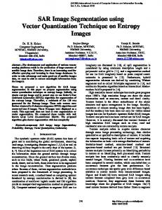
denotes the kth transition and τ is the decrease ratio. As it was pointed out in [Kirkpatrick et al (1983)], in order to estimate the global minimum of energy functions, τ must be close to 1. In this study τ = 0.95. Figure 3 shows the final result of the segmentation.

. (a) (b) Figure 3. (a) Final result of the segmentation, (b) Original image with boundary line. 4 Conclusions A scheme for image segmentation has been described, in which an attempt is made to use spatial information to overcome the weaknesses of purely statistical methods. This method consists in three main steps: quadtree smoothing, centroid clustering and boundary estimation. The segmentation depends on the boundary shape and downward propagation of errors. The low resolution classification is statistical but is based on a local centroid algorithm, which do not requires a priori information. To assure a minimum of errors in the lowest level and in order to prevent the propagation of errors, we classify the pixels of the boundary by using three differents criteria: the nearest class mean, Mahalanobis distance and Potts model. Markov random fields theory offers an opportunity to overcome signal-to-noise ratio conditions typical of SAR images. Experimental results have been presented which bear out theoretical expectations and demonstrate the power of the method. Some of the perspectives to continue this study are: a) To apply a probabilistic relaxation in order to obtain low resolution segmentations; b) In the highest

1151

Anais IX Simpósio Brasileiro de Sensoriamento Remoto, Santos, Brasil, 11-18 setembro 1998, INPE, p. 1145-1152.

level, classifications can be made by using an binary scheme (Markovian Ising model). Extensions to texture segmentation are foreseen. References Arellano O. Método de estructuras de árbol (quadtree) para la segmentación de imágenes de percepción remota, Thesis of Master, México, 1997. Descombes X.; Moctezuma M.; Maitre H.; Rudant J-P. Coastline detection by a Markov segmentation on SAR images, Signal Processing No. 55, 1996, pp. 123-132. Devijver, P.A.; Kittler, J. Pattern Recognition: A Statistical Approach, London, Prentice Hall, 1983. Geman S.; Geman D. Stochastic relaxation, Gibbs distribution and the Bayesian restoration of images, IEEE Trans. Pattern Anal. Machine Intell., vol. 6, No. 6, 1984, pp. 721-741. Kirkpatrick S.; Gellat C.; Vecchi M. Optimization by simulated annealing, Science, No. 220, 1983, pp. 671-680. Schneier M. Linear time calculations of geometric properties using quadtrees, TR-770 Computer Science Center, University of Maryland, 1979. Spann M.; Wilson R. A quadtree Approach to Image Segmentation that Combines Statistical and Spatial Information, Patt. Rec. 18, 1985, pp. 257-269. Wilson R. From Signals to Symbols- the Inferential Structure of Perception, Proc. IEEE COMPINT-85, Montreal, 1985, pp. 221-225. Wilson R.; Spann M. Image Segmentation and Uncertainty, Research Studies Press LTD, England, 1988.

1152