animation of the original movement, a second SOM was trained on the appearance of the ... free throw shot and is often performed in the presence of defenders.
International Journal of Computer Science in Sport – Volume 9/Edition 1
www.iacss.org
Self-Organising Maps: An Objective Method for Clustering Complex Human Movement Peter Lamb, Roger Bartlett, Anthony Robins University of Otago, Dunedin, New Zealand
Abstract In this study self-organising maps (SOM) were used to classify the coordination patterns of four participants performing three different types of basketball shot from different distances. The shots were the free throw, the three-point and the hook shot. The free throw and three-point shot were hypothesised to be more similar to one another than to the hook shot. The first analysis involved an analysis of trial trajectories visualised on a U-matrix. Two of the participants, unexpectedly, showed more similarity between the three-point shot and the hook shot, instead of the free throw. Where the first analysis was useful in showing aspects of the movement that were not obvious from viewing the computer animation of the original movement, a second SOM was trained on the appearance of the original trajectories and used to produce an output that shows the variability in coordination between all trials in the study. The second SOM showed groupings of the three shooting conditions which were unexpected. The second SOM technique may provide a more objective method than visual technique analysis for explaining movement patterning and structuring practice routines. KEYWORDS: NEURAL BASKETBALL.
NETWORKS,
KOHONEN,
SOM,
COORDINATION,
Introduction The data used for this study were generated from four players performing three different types of basketball shot from different distances. The shots were the three-point shot, the free throw and the hook shot. The free throw and three-point shot were hypothesised to be more similar to one another than to the hook shot. A free throw is commonly awarded when an offensive player is fouled during shooting. Each foul usually results in the offended player being awarded two free throw shots, which makes the free throw shot an important skill. The three-point shot is more strategic; the probability of successfully scoring with this shot is much less but the reward is higher. The three-point shot is taken from further away than the free throw shot and is often performed in the presence of defenders. Subsequently, the threepoint shot is almost always performed as a jump shot, both to afford more power for the shot and to release the ball higher thus reducing the chance of being blocked. During the study, the hook shot was performed starting with the player’s back to the net then turning and shooting with a one-handed release. The hook shot has a lower percentage success rate but, because of the release point, it is a difficult shot to defend. A good hook shot involves the shooter’s body
20
International Journal of Computer Science in Sport – Volume 9/Edition 1
www.iacss.org
being positioned between the ball and the defender. Typically the hook shot is used as a last resort and, therefore, occurs less frequently than the other two shots. A likely practice routine would reflect the hook shot’s infrequent use. The hook shot is often assumed to be a different movement pattern compared to the similar patterns used for the free throw and the three-point shot, which are often thought of as modifications of the ‘set shot’ movement pattern. Consider why these assumptions exist. The observational learning literature suggests the motion of distal segments as one of the most influential factors when learning new skills (Hodges, Williams, Hayes, & Breslin, 2007). The typical one-handed release of the hook shot makes the kinematics of the distal segments a plausible explanation for its distinction as a unique shot. If such visual information negatively influences the observer, the opportunity exists for a new method of structuring practice and thinking about movement patterning to come to light. The purpose of this study was to show that SOMs are an objective tool for movement analysis. Methods Data Collection and Processing A 12-camera, three-dimensional motion capture system (Motion Analysis Corporation Inc, Santa Rosa, CA, USA) was used to collect the data for this study. Using post-processing software (Visual3D, C-Motion), a 12-segment body model was established. Based on the Euler convention, motion in the sagittal plane for the right and left ankles, knees, hips (Bell, Pedersen, & Brand, 1990) and shoulders (Rab, Petuskey, & Bagley, 2002) were processed for the SOM analysis. Trials were time normalised to 101 data points. Within each trial, each variable was range normalised to maximum and minimum values of +1 and -1, respectively. The trials were appended one after the other to create one block of data used for training the neural network. SOM Outline The SOM can be thought of as a layer of nodes with associated weight vectors, fed forward by a layer of inputs. Weight vectors of the map nodes are adjusted based on an unsupervised learning strategy to represent relevent information in the input. The output node whose weight vector has the smallest Euclidean distance to a given input is declared that input’s best matching node. Convergence to the input is acheived by iteratively updating the weights of the best matching node and its neighbours, within a specified radius, according to the neighbourhood function and learning rate (Kohonen, 2001). Because of such non-linear properties, the SOM is able to remove redundancies in high-dimensional input data and produce a low-dimensional mapping of the output while preserving topological relationships in the data. The neighbourhood function effectively allows local interactions between map nodes to coalesce into states of global order and to achieve self-organisation. Network Architecture The SOM toolbox for MATLAB was integrated into the software tool (Vesanto, Himberg, Alhoniemi, & Parkankangas, 2000) for the analysis. A PCA-based initialisation process was used to create a two-dimensional hexagonal lattice output map (Table 6). The neighbourhood sizes were selected according to the principal components of the data (Barton, Lees, Lisboa, & Attfield, 2006).
21
International Journal of Computer Science in Sport – Volume 9/Edition 1
www.iacss.org
A second SOM, inspired by Barton (1999), was trained on the trajectories from the original SOM. Inputs for the second SOM were created from projecting the weight vectors into weight space using Sammon’s mapping (Sammon, 1969). The two-dimensional coordinates of each consecutive best matching node were used to create an input vector representative of an individual trial. This process was repeated for the best matching nodes of all trials in the study. The result of the second map is a SOM in which each trial can be represented by one node on the output map and, therefore, a clustering of all the trials in the dataset can be visualised more easily. In what follows we will refer to the original SOM as the phase SOM and the second SOM as the trial SOM. Table 6: SOM training parameters and quality measures
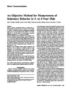
Analysis We chose to use the U-matrix (Figure 6(a)) to visualise the output of the phase SOM. Trajectories connecting nodes on the U-matrix that best represent the input were used to visualise the multi-segment coordination performed by the participants. The nodes in Region A of the U-matrix represent the preparation phase of the shot. Region B represents the extension phase where the player generates power for the release. Region C represents the final release phase of the movement. Typical movement patterns activate nodes in Region A, ascend up the map through Region B and end at the release phase in Region C. Movements that were patterned uniquely, activated nodes in Region D. Clusters of data can be identified on the U-matrix with blue ‘distance cells’ which are evidence of similar data among neighbouring nodes. Orange and red distance cells represent larger Euclidean distances between neighbouring nodes and therefore outline borders between clusters.
22
International Journal of Computer Science in Sport – Volume 9/Edition 1
www.iacss.org
Figure 6: a) U-matrix and movement phases: A Preparation, B Extension, C Release, D Unique coordination; b) Preparation phase; c) Extension phase; d) Release phase.
The phase SOM analysis uses the trajectory of the best matching nodes through the time series of each trial to compare various trials simulated on the same U-matrix visualisation (Lamb, Bartlett, Robins, & Kennedy, 2008). The orange trajectories shown on the U-matrix (Figure 7(a), (c) and (e)) give a representation of the order of the best matching nodes with respect to time. However, the trajectory can potentially be misleading as it gives the impression that the best matching nodes move fluidly through the U-matrix. Visualising trials with just the best matching nodes highlighted in white on black shows the discontinuity on the U-matrix for this dataset. Figure 7 ((b), (d) and (f)) shows these hit histograms with best matching nodes shown as white patches with their size increasing as the frequency of hits increases. For these nodes to stand out the rest of the U-matrix is blacked out. Sammon’s mapping was used to visualise the trial SOM because the map size was small with an accordingly small topographical error (Table 6). Each trial in the dataset was assigned a best matching node which was shown on the output map (Figure 11). The text at each node represents the type of shot, the colour of the text identifies the player and the size of the text increases as the hit frequency increases. The lateral connections between nodes represent the Euclidean distance between them. Results Phase SOM analysis The trajectories for the three-point shot and free throw are visually similar in Regions A and C of the U-matrix, suggesting that the coordination patterns in the preparation and release phases were similar. The trajectories differ in the middle area of the map, in Region B, in which the three-point shot moves closer to the right edge of the map (Figure 2(a)) than the trajectories for the free throw (Figure 2(c)). The trajectory for the hook shot (Figures 2(e), (f)) is qualitatively different from the other two shots for Player 1. The main visual difference in the trajectories was seen as the trajectory moves diagonally up and across the U-matrix in Region C. 23
International Journal of Computer Science in Sport – Volume 9/Edition 1
www.iacss.org
Figure 7: Player 1, a) Three-point shot trajectory, b) Three-point shot hits, c) Free throw trajectory, d) free throw hits, e) hook shot trajectory, f) hook shot hits, g) U-matrix with movement phases.
For Player 2 (Figure 8), the preparation phase for the three-point shot and the free throw are almost identical, occupying many of the same nodes and clustering similarly. During the release phase, the three-point shot moves diagonally up and to the left from the right edge of the map in Region C (Figure 8(a), (b)), similarly to the three-point shot and free throw of Player 1. The diagonal movement on the U-matrix of the free throw is not as long or as consistent as the three-point shot (compare Figure 8(a) with Figure 8(c)). The hook shot (Figure 8(e), (f)) is, again, qualitatively different from the other two shots. Unlike all other shooting conditions for all other players, the best matching node trajectory for the hook shot for Player 2 does not always progress upwards on the U-matrix. The hit histogram in Figure 8(f) shows the best matching nodes for most of the movement are within two brightly coloured borders in Region D of the U-matrix. This is different from any other shot in the dataset.
Figure 8: Player 2, a) Three-point shot trajectory, b) ) Three-point shot hits, c) Free throw trajectory, d) free throw hits, e) hook shot trajectory, f) hook shot hits, g) U-matrix with movement phases.
24
International Journal of Computer Science in Sport – Volume 9/Edition 1
www.iacss.org
The best matching node trajectories for Player 3 are similar for the three-point shot and the free throw (Figure 9(a), (c)). The hit histograms show a large discontinuity as the movement transitions from preparation to release (see Figure 9(b), (d)). The trajectory jumps from Region A to a series of about three different nodes in Region D before jumping into Region C for the release phase of the shot. The jump into Region D is different from any of the other shots in the dataset. The hook shot is visually much different from the three-point shot and the free throw; it stays within Region D, without jumping across any borders, and along a very consistent trajectory of nodes (Figure 9(e)).
Figure 9: Player 3, a) Three-point shot trajectory, b) ) Three-point shot hits, c) Free throw trajectory, d) free throw hits, e) hook shot trajectory, f) hook shot hits, g) U-matrix with movement phases.
For Player 4, the trajectories for the preparation phase of each shot are different. The threepoint (Figure 10(a), (b)) and hook shot (Figure 10(e), (f)) best matching nodes were in Region A, as expected, whereas the free throw (Figure 10(c), (d)) began in Region D. In Region B, the three-point shot and hook shot trajectories travel to the left of the bright blue border near the right edge of the U-matrix (highlighted in yellow in Figure 10(g)) whereas the free throw travels to the right of the border. The release, shown in Region C, of the threepoint shot and the free throw are quite similar, as shown in Figure 10(a) and (c). The release of all three shots of Player 4 resemble the release of Player 1. The trajectories for the threepoint shot and the free throw move above the bright blue border in the middle of Region C, while the trajectory for the hook shot moves below the border.
25
International Journal of Computer Science in Sport – Volume 9/Edition 1
www.iacss.org
Figure 10: Player 4, a) Three-point shot trajectory, b) ) Three-point shot hits, c) Free throw trajectory, d) free throw hits, e) hook shot trajectory, f) hook shot hits, g) U-matrix with movement phases.
Trial SOM analysis Starting with Player 1 (blue text in Figure 11), the three-point shot and hook shot occupy nodes at the left edge of the map which makes the two shots second nearest neighbours. The free throw hits a region toward the bottom of the map, located more closely to different shot types of different players than to other shots by Player 1. As was shown in the previous section in Figure 7 and 3, the coordination patterns for each respective shot for Player 1 and Player 4 (red) are similar. Also the three-point shots and free throws of Player 2 (green) were clustered near the three-point shot of Player 1 (compare Figure 11 with Figure 7 and Figure 8). The three-point shot and free throw for Players 2 and 3, respectively, are second nearest neighbours with a noticeably short Euclidean distance between them (compare trajectories in Figure 8(a) and (c) and Figure 9(a) and (c)). Most of the hook shots for Player 2 were isolated toward the top right corner of the map. Higher variability within this shooting condition is evident by the distribution of hits across six nodes. Three other shooting conditions occupy more than one node (Player 2 three-point shot and free throw and Player 3 free throw); however, the Euclidean distance spanned by the hook shots of Player 2 show this to be the most variable shooting condition in the dataset.
26
International Journal of Computer Science in Sport – Volume 9/Edition 1
www.iacss.org
Figure 11: Sammon's mapping of trial SOM. Player 1 is shown in blue, Player 2 in green, Player 3 in red and Player 4 in cyan.
Figure 9 showed the three-point shot and free throw of Player 3 (red) to appear similar to, although distinct from, other shots in the dataset. The hook shot occupied a small area in Region D in Figure 9, which was also distinct from other shots in the dataset. Both of these observations are apparent in Figure 11 (in red). The three-point shot and free throw are separated by only one node and the hook shot is isolated in the top right corner of the map. The free throw of Player 4 (cyan) is another shot that is clustered away from the rest of the data, in this case the bottom right corner of the map. The three-point and hook shots are shown to be more similar to each other than to the free throw; these shots are also more similar to the three-point and hook shots of Player 1 that they are to the free throw of Player 4. Finally, notice that the three-point shot appears to be the most similar shooting condition among the players, and the hook shot the least similar. Discussion The Jump Hook Qualitatively, Player 1 supported the hypothesis that the three-point shot (Figure 7(a)) and the free throw (Figure 7(b)) would be most similar, but only for the preparation and release phases. Although all time frames of the movement were weighted equally, the trial SOM classified the data for the three-point shot and hook shot in the extension phase to be a larger contributor to overall similarity, partly because of a slight delay at mid-flight between lower and upper body extension in these shots. Overall, the trial SOM showed the lowest variability between the three-point and the hook shots; during the late extension phase and the beginning of the release of the shot, the three-point shot showed more similarity with the hook shot than with the free throw. For the three-point (Figure 10(a)) and hook (Figure 10(e)) shots, many similar nodes were activated in the extension phase (Region B, Figure 10(g)) for Player 4, adding further
27
International Journal of Computer Science in Sport – Volume 9/Edition 1
www.iacss.org
evidence that the kinematics involved in the jump in these two shots contribute to the data for each of these shooting conditions being more similar to each other than to the free throw, which does not involve a jump. The release phase of the three-point shot (Figure 10(a)) and free throw (Figure 10(c)) showed more similarity on the U-matrix. This was expected since the three-point shot and the free throw are two-handed shots, whereas the hook shot is a onehanded shot. Computer animations showed that the noticeable difference between the threepoint shot and the free throw for Player 4 was the in-phase extension of the upper and lower body; for the free throw the knees and hips reached maximum extension while the upper arms continued to flex and the elbows and ankles continued to extend. The upper arms then stopped, leaving both the ankles and elbows still extending – a somewhat atypical sequence. This sequence is shown on the U-matrix by nodes between the edge of the map and the rightmost brightly coloured border in Region B (Figure 10(c)). Player 4's free throw was the only shot for any of the players to activate these nodes. The overall similarity of the movement patterns used for the three-point shot and the hook shot is verified in Figure 11. The close proximity of best matching nodes for the release phase of the hook shot for Players 1 and 4 suggest high similarity between these players for the hook shot release. The short Euclidean distance for the hook shots between Players 1 and 4 on the trial SOM (Figure 11) suggests further that the hook shots of these two players are similar. The high dimensionality of the time series data for these throws makes an in-depth, visual analysis of coordination difficult using conventional methods. Research into the information attended to in visual demonstrations has shown that the kinematics of distal segments (arms) has a greater impact than the kinematics of more proximal segments (trunk) in skill acquisition (Hodges et al., 2007). This may be used as evidence suggesting that certain information biases the movement analyst. Since the major difference associated with the hook shot compared to the other two shots is the one-handed release, one could speculate that the movement of the distal segments over-influence the analyst into classifying the hook shot as a completely different movement. If this is the case, the SOM might provide an objective method for analysing human movement for movement analysts and coaches. The standing hook Only the shots of Players 2 and 3 were clustered on the trial SOM in support of the hypothesis that the three-point shot and free throw would show less variability between them than when compared to the hook shot. Qualitatively, the three-point shot and free throw, for both Player 2 (Figure 8(a), (c)) and Player 3 (Figure 9(a), (c)), were similar to each other for not only the preparation and release phases of the movement, as for Player 1, but also the extension phase of the movement. The hook shots were qualitatively different for each phase and occupied Region D on the U-matrix (Figure 8(e) and Figure 9(e)). Unique to Players 2 and 3 was that their hook shots lacked a significant jump along with an early release of their three-point shot. The jumping kinematics that separated the three-point shot and the free throw for Players 1 and 4 were much less pronounced for Players 2 and 3, reflected in the short Euclidean distance between the three-point shot and free throw on the trial SOM (Figure 11, Players 2 and 3). Conclusions The phase SOM drew our attention to aspects of the movement that were not obvious from more traditional approaches, such as visual analysis of the original movement, or from multiple time series data. Characteristics of the movements found by analysis of the phase 28
International Journal of Computer Science in Sport – Volume 9/Edition 1
www.iacss.org
SOM were summarised on a single output map using the trial SOM. In several cases, the SOM output and our natural inclinations as movement analysts did not agree; SOMs thus proved to be a useful tool in our analysis of coordination. The movement analyst might be distracted by visual information in the movement; the SOM might provide a more objective method for explaining movement coordination. In particular, the trial SOM approach may be useful for a gaining a more global representation of the dataset and thus neatly summarise the relationships between a set of coordination patterns. References Barton, G. (1999). Interpretation of gait data using Kohonen neural networks. Gait & Posture, 10, 85-86. Barton, G., Lees, A., Lisboa, P., & Attfield, S. (2006). Visualisation of gait data with Kohonen self-organising neural maps. Gait & Posture, 24, 46-53. Bell, A. L., Pedersen, D. R., & Brand, R. A. (1990). A comparison of the accuracy of several hip center location prediction methods. Journal of Biomechanics, 23(6), 617-620. Hodges, N. J., Williams, M. A., Hayes, S. J., & Breslin, G. (2007). What is modelled during observational learning? Journal of Sports Sciences, 25(5), 531-545. Kohonen, T. (2001). Self-organizing maps (3rd ed.). Berlin, Germany: Springer-Verlag. Lamb, P., Bartlett, R. M., Robins, A., & Kennedy, G. (2008). Self-Organizing Maps as a tool to measure movement variability. International Journal of Computer Science in Sport, 7(1), 28-39. Rab, G., Petuskey, K., & Bagley, A. (2002). A method for determination of upper extremity kinematics. Gait and Posture, 15, 113-119. Sammon, J. W. (1969). A nonlinear mapping for data structure analysis. IEEE Transactions on Computers, C-18(5), 401-409. Vesanto, J., Himberg, J., Alhoniemi, E., & Parkankangas, J. (2000). SOM Toolbox for MATLAB 5 (No. A57). Helsinki, Finland: Helsinki University of Technology.
29