MSU GARAGe for their suggestions and critical feedback, particularly Terry Dexter for his thoughts on the dynamics of mask bits on the GA chromosome.
Simultaneous Feature Extraction and Selection Using a Masking Genetic Algorithm Michael L. Raymer1,2, William F. Punch2, Erik D. Goodman2,3, Paul C. Sanschagrin1, and Leslie A. Kuhn1 1
Protein Structural Analysis and Design Laboratory, Department of Biochemistry, Genetic Algorithms Research and Applications Group, Department of Computer Science, 3 and Case Center for Computer-Aided Engineering and Manufacturing, Michigan State University, East Lansing, MI 48824.
2
Abstract Statistical pattern recognition techniques classify objects in terms of a representative set of features. The selection of features to measure and include can have a significant effect on the cost and accuracy of an automated classifier. Our previous research has shown that a hybrid between a k-nearest-neighbors (knn) classifier and a genetic algorithm (GA) can reduce the size of the feature set used by a classifier, while simultaneously weighting the remaining features to allow greater classification accuracy. Here we describe an extension to this approach which further enhances feature selection through the simultaneous optimization of feature weights and selection of key features by including a masking vector on the GA chromosome. We present the results of our masking GA/knn feature selection method on two important problems from biochemistry and medicine: identification of functional water molecules bound to protein surfaces, and diagnosis of thyroid deficiency. By allowing the GA to explore the effect of eliminating a feature from the classification without losing weight knowledge learned about the feature, the masking GA/knn can efficiently examine noisy, complex, and high-dimensionality datasets to find combinations of features which classify the data more accurately. In both biomedical applications, this technique resulted in equivalent or better classification accuracy using fewer features.
1
Introduction
The selection of appropriate features is an important precursor to most statistical pattern recognition methods. A good feature selection mechanism helps to facilitate classification by eliminating noisy or non-representative features that
can impede recognition. Even features which provide some useful information can reduce the accuracy of a classifier when the amount of training data is limited [1-3]. This so-called “curse of dimensionality”, along with the expense of measuring and including features, demonstrates the utility of obtaining a minimum-sized set of features that allow a classifier to discern pattern classes well. Some classification rules, such as the k-nearestneighbors (knn) rule, can be further enhanced by multiplying each feature by a weight value proportional to the ability of the feature to distinguish among pattern classes. This feature weighting method is a form of feature extraction – defining new features in terms of the original feature set to facilitate more accurate pattern recognition. Feature selection and extraction, in combination with the k-nearestneighbors classification rule, have been shown to provide increased accuracy over the knn rule alone, and can aid in the analysis of large datasets by isolating combinations of features that distinguish well among different pattern classes [4,5]. Genetic algorithms (GA’s) have been applied to the problem of feature selection by Siedlecki and Sklanski [6]. In their work, the genetic algorithm performs feature selection in combination with a knn classifier, which is used to evaluate the classification performance of each subset of features selected by the GA. The GA maintains a feature selection vector consisting of a single bit for each feature, with a 1 indicating that the feature participates in knn classification, and a 0 indicating that it is omitted. The GA searches for a selection vector with a minimal number of 1’s, such that the error rate of the knn classifier remains below a given threshold. Later work by Punch et al. and Kelly & Davis expanded this approach to use the GA for feature extraction [4,5].
1
Instead of a selection vector consisting of only 0’s and 1’s, the GA manipulates a weight vector, in which a discretized real-valued weight is associated with each feature. Prior to knn classification, the value of each feature is multiplied by the associated weight, resulting in a new set of features which are linearly related to the original ones. The goal of the genetic algorithm is to find a weight vector which minimizes the error rate of the knn classifier, while reducing as many weights as possible to zero. We have previously applied the GA/knn feature extraction method to the problem of predicting conserved water molecules in protein ligand binding, an important problem in protein and drug design [7]. In this paper we describe an expanded approach in which the GA is used to perform simultaneous feature selection and feature extraction. This approach uses both a feature weight vector and a masking, or selection, vector on the GA chromosome. Feature weights are real-valued, while the mask values are either 0 or 1. Each feature is multiplied by both its weight value and its mask value prior to classification by a knn classifier. In this approach, the GA can test the effect of eliminating a feature completely from the classification by setting its mask value to zero without reducing the associated feature weight to zero. This allows the feature to be re-introduced later without losing previously-learned weight information. Results of this method are compared with previous feature extraction results for complex, noisy datasets from biochemistry and medicine.
2
Methods
2.1
K-nearest-neighbors classification
feature space. Each axis in this space represents one feature being considered by the classifier. Once the training data are plotted, the unknown object is plotted in the feature space according to the observed values of its features. The unknown is then typically classified according to the majority class of its k nearest neighbors. In the figure, three of the five nearest neighbors (shaded gray) are of class 2, so the unknown is classified as belonging to class 2. We used the branch and bound knn algorithm [8] to improve the efficiency of the knn by reducing the number of distance calculations involved in finding the nearest neighbors of the unknown pattern. In the weighted knn classifier, the feature values of the training patterns and the unknown pattern are multiplied by the corresponding weight values prior to classification. The result is that the feature space is expanded in the dimensions associated with highly weighted features, and compressed in the dimensions associated with less highly weighted features, as shown in Figure 1b. This allows the knn classifier to distinguish more finely among patterns along the dimensions associated with highly-weighted features. In the figure, the classification of the unknown pattern changes to class 3 after feature scaling has been applied, since four of the five nearest neighbors (shown in gray) of the unknown are now samples from class 3. If a feature weight is zero, then all the values in the corresponding dimension are reduced to zero, and that feature effectively drops out of the classification. For our experiments, all features are normalized over the range [1.0-10.0] prior to
a. Class 2 Class 3
? ?
Feature 1 b. Compressed
A k-nearest-neighbors classifier is used to evaluate each weight set evolved by the GA. This allows a great deal of generality in the classification, because the knn classification method does not depend on the data following any particular distribution, unlike many other classifiers which assume a multivariate Gaussian distribution of the feature values. The algorithm used in knn classification is simple. First, training patterns are plotted in a ddimensional feature space, where d is the number of features being used for the classification. These training patterns are plotted according to their observed feature values along the corresponding feature axes, and labeled with their known classification. For example, Figure 1a. shows training patterns from 3 classes plotted in a 2-dimensional
Feature 2
Class 1
?
Figure 1: Scaling the KNN algorithm. 2
Unknown
weighting and classification, in order to avoid an implicit weighting of features which have different ranges in values. For some applications, it is not practical to obtain an equal number of training patterns of each class. In diagnosis of rare diseases, for example, there are far more patients who do not have the disease in question than those who do. If every patient’s medical information is used to train a knn classifier to classify a patient as “healthy” or “ill”, it is likely that there will be a bias towards “healthy” classifications, simply because there will be more “healthy” training points to potentially contribute to the classification. We employ two distinct approaches to eliminate voting bias due to unbalanced training data. The first approach is to equalize the number of examples of each class by stratifying the randomized selection of the training data. All available examples of the least common class are included in the training set, along with an equal-sized, randomly selected set of examples from the more common classes. In the second approach, all examples of each class are included in the training set. Bias is avoided by implementing class-balanced voting that weights the votes from members of each class such that the sum of weighted votes over all members of a class is equal for all classes. This approach was successfully applied by Salamov and Solovyev in their knn approach to the prediction of protein secondary structure [9]. 2.2
The genetic algorithm
The chromosome for the masking GA/knn is composed of two parts. The first part consists of one real-valued weight for each of the features being considered. In this implementation, the weights range from 0 to 100 and are represented as 32-bit, unsigned, floating-point numbers. The second part of the chromosome is the feature masking vector. Two approaches were used in constructing the mask vector. In the first method, a single mask bit was associated with each feature. If the bit associated with a certain feature was set to zero, then the feature was omitted from the knn classification. Otherwise, the appropriate weight was applied to the feature as described above, and the feature participated in the knn classification process normally. Since this technique places significant importance on a single bit of the GA chromosome, a second method was devised to reduce the large phenotypic variation associated with a single-bit genotypic change in the mask bits. In this second approach, m mask bits were associated
with each feature, and the feature participated in classification only if the number of 1’s among these m bits was greater than or equal to m/2. Under both methods a feature could also be removed from consideration if its weight value started at or was reduced to zero; however this unlikely event did not occur in any of the experiments reported here. Chromosomes are evaluated by applying the anti - fitness ( weight set ) =
C pred (# incorrect predictions)
+ C bal (difference in error rate among classes) + C vote ( # missed votes)
+ C mask ( # unmasked features)
Figure 2: Overview of the GA objective function. The constants applied to each term are adjusted empirically based on run results. For typical runs, the contribution to the overall anti-fitness from incorrect predictions is ~72-78%, from difference in error rate among classes, ~10%, from missed votes, ~10%, and from unmasked features ~2-8%, depending upon the number of features masked. weight and mask vectors to the feature set, and performing classification on a set of patterns of known class with a feature-weighted knn classifier. The fitness assigned to a chromosome is computed in several parts. The two most important parts of the fitness function are the error rate of the knn classifier on the known test data, and the number of features which were used in the classification. This allows the masking GA/knn to simultaneously drive toward greater classification accuracy and the use of fewer features. In addition, the number of incorrect votes in the knn classification process is used to smooth the fitness function and provide additional guidance for the GA. A balance term is also introduced to prevent bias introduced by unequal numbers of test patterns in different classes; this is particularly important in the absence of class-balanced voting. For example, if a dataset consists of 95 patterns from class A and only 5 from class B, the balance term prevents the GA from training the knn to always predict class A and thus achieve a 5% apparent error rate. Since the GA engine we are using, GAUCSD [10], is a function minimizer, anti-fitness is measured rather than fitness. The anti-fitness function being minimized is summarized in Figure 2.
3
The available data are partitioned into several sets for each GA/knn run, with or without masking. First, the data, all of which have known class, are partitioned into a training set and a holdout set for external testing. The training data are then further partitioned into a knn training set, used to populate the knn feature space with voting examples, and another set to be sequentially classified by the weighted knn to provide feedback to the GA on the effectiveness of the current weight set. Once the GA/knn training has converged or reached a fixed generation limit, the best weight set identified is used along with a weighted knn algorithm to perform an unbiased classification on the holdout test set. GA training runs were typically executed for 100 or 200 generations, with a population size of 200. 2.3
Experiments on biochemical data
Most experiments were performed on a set of data describing the environments of water molecules bound to protein surfaces, which are important for protein function. Water molecules in this dataset belong to one of two classes: those displaced from the protein surface when the protein binds another molecule, such as a drug, and those that are conserved. Five features characterizing the local environment of water molecules in 20 independently-solved, unrelated protein structures were calculated. These features measure characteristics such as the number of protein atoms packed around the water molecule, the number of hydrogen bonds between the water molecule and the protein, the thermal mobility of the water molecule measured in two different ways, and the frequency with which the atoms surrounding the water molecule tend to bind water molecules in another database of proteins [11]. Since there were significantly more conserved than displaced water molecules, the dataset was balanced by randomized selection as described in section 2.1. The result was a set of 2728 water molecules that were used for training and testing data in subsequent experiments. 2.4
Experiments on medical data
A second set of experiments was done to determine the ability of the masking GA/knn to perform feature selection on a dataset of higher dimensionality than the waters data. For these experiments, we selected a medical dataset consisting of 21 clinical test results for a set of patients being tested for thyroid dysfunction. The training set is composed of test results for 3772 cases from the year
4
1985, while the testing data consists of the 3428 cases from 1986. The goal is to determine whether or not a patient is hypothyroid. Previous analyses of this data have shown that traditional classifiers, including discriminant analysis, Bayes classifiers, and neural networks can classify this dataset well using all available features [12,13]. Our goal was to determine if the masking GA/knn can be trained to provide comparable classification performance with a significant reduction in the number of clinical tests required. The number of samples of each class is highly unbalanced in both the training and testing data. The training set contains 3487 negative (non-hypothyroid) samples, and 284 positive samples. The testing data consists of 3177 negative samples and 250 positive samples. Due to this imbalance, class-balanced voting was used for experiments with unweighted knn classification, and with the masking GA/knn. Masking runs were done using 15 mask bits and one 32-bit floating point weight for each feature, for a total chromosome length of 987 bits.
3
Results
3.1
Classification of protein-bound water molecules
The goals of our research on protein-bound water molecules are twofold. First, we would like to be able to classify whether specific water molecules are more likely to be conserved or displaced upon ligand binding. We have previously shown that a knn classifier in combination with a GA feature extractor can achieve significantly improved classification for bound waters, compared to unweighted knn classification, and linear and quadratic discriminant analysis [7]. We have also used a genetic programming (GP) approach to apply a polynomial function, rather than a linear coefficient, to each feature prior to knn classification [14]. The GP approach showed an improved performance due to the ability to discover non-linear relationships between features, but was more prone to the problem of “overfitting” – finding overly specific classification rules that perform well on the training data, but do not generalize well to new data. The second goal of our protein-water research is to elucidate the determinants of water binding on the protein surface – that is, which features are important for binding, and which features are less relevant. The
inclusion of mask bits in the GA chromosome, and subsequent feature selection results, succeed in identifying combinations of features which distinguish well between conserved and displaced water molecules. By analysis of these results we can gain insight into which chemical and structural factors are more important contributors to the conservation of water molecules in ligand binding. GA runs for feature extraction alone, then extraction in combination with selection, were done using jackknife cross-validation [15]. In each of these jackknife tests, the 2728 available water molecules were partitioned into training and holdout-testing sets. The accuracy of the classifier is observed and averaged over several runs with similar initial conditions, but different balanced but otherwise randomly-selected training and testing sets. For feature extraction runs, the training set contained 2296 waters, 1148 of which were known-class waters used to populate the knn feature space, and 1148 of which were knowns classified to provide feedback to the GA. The other 432 waters, treated as unknowns, composed the holdout test set. For masking runs, a similar training set of 2300 waters was divided equally between knn population and weight tuning, and the holdout-test set had 428 waters. Table 1 shows the unbiased holdout test results of several experiments using only feature extraction. The value of k was set to 39 for all runs after being optimized as described in [7]. The classifier’s conserved water, displaced water, and overall predictive accuracy are shown, along with the weights applied to each feature. In order to reduce the amount of redundant information on the chromosome in the form of linearly-related weight sets, a parsimony term was added to the fitness function to reward weights of smaller magnitude by penalizing each weight set according to the sum of its weights.
Cons 81.02% 81.94 74.54 75.46 77.31 69.44 67.59 72.22 68.98 71.76
Predictive Accuracy Disp Total 57.41% 69.21% 55.09 68.52 61.57 68.06 59.72 67.59 57.41 67.36 62.50 65.97 63.43 65.51 56.48 64.35 58.80 63.89 52.31 62.04
Individual weight sets were then normalized to sum to 1.0 to facilitate comparison between weights from different runs.
Masking runs were done using the same weighting scheme as the extraction-only runs, with the addition of single mask bit per feature to the GA chromosome. An additional feature, NMOB, reflecting atomic mobility as a combination of atomic occupancy (OCC) and temperature factor (BVAL), was included in these runs to assess whether NMOB or BVAL provided more classification power. The holdout test results of the masking runs are shown in Table 2. Weights of zero indicate that a feature was masked and not used in the knn classification.
Weight sets with two or three features masked performed equivalently in classification accuracy to weight sets including all four features in previous runs (Table 1). Masking of weights was consistent from run to run, with different masking patterns tending to be associated with different classification balance and accuracy. It is possible to classify bound water molecules as conserved or displaced with 68% accuracy and good balance using only three features, atomic density, B-value, and number of hydrogen bonds, saving the need to measure atomic hydrophilicity and mobility values.
NADN 0.149 0.161 0.031 0.061 0.055 0.168 0.056 0.006 0.094 0.097
Feature Weights NAHP NBVAL 0.276 0.229 0.328 0.173 0.323 0.255 0.051 0.613 0.235 0.383 0.116 0.303 0.360 0.222 0.347 0.330 0.190 0.224 0.040 0.518
NHBD 0.346 0.337 0.391 0.275 0.328 0.412 0.361 0.317 0.492 0.345
Table 1: Results of GA feature extraction runs with parsimony. Prediction accuracy for conserved (Cons) and displaced (Disp) water molecules, as well as the total prediction accuracy over both classes, are shown. Also shown are the final weights found by the genetic algorithm for each feature: normalized atomic density (NADN), normalized atomic hydrophilicity (NAHP), normalized B-value (NBVAL), and normalized hydrogen-bond count (NHBD). For further details about these features and the GA/knn feature extractor, see [7].
5
Cons 67.29% 64.02 62.62 68.22 64.95 65.42 61.68 64.02 65.42 64.02 66.36 63.55 61.68 59.35 64.95
Predictive Accuracy Disp Total 69.63% 68.46% 70.56 67.29 70.09 66.36 62.62 65.42 65.89 65.42 64.95 65.19 66.36 64.02 64.02 64.02 61.68 63.55 62.62 63.32 59.35 62.85 60.28 61.92 62.15 61.92 63.08 61.21 56.07 60.51
NADN 0.175 0.142 0.000 0.000 0.000 0.000 0.166 0.000 0.000 0.000 0.000 0.180 0.000 0.191 0.158
NAHP 0.000 0.219 0.373 0.000 0.000 0.400 0.000 0.000 0.000 0.000 0.000 0.000 0.000 0.000 0.254
Feature Weights NBVAL NHBD 0.491 0.335 0.437 0.000 0.414 0.000 0.130 0.536 0.581 0.419 0.263 0.000 0.463 0.371 0.470 0.153 0.278 0.000 0.752 0.248 0.575 0.425 0.307 0.514 0.505 0.495 0.333 0.476 0.279 0.309
NMOB 0.000 0.202 0.213 0.334 0.000 0.337 0.000 0.377 0.722 0.000 0.000 0.000 0.000 0.000 0.000
Table 2: Feature extraction and selection results. Prediction accuracy for conserved (Cons), and displaced (Disp) waters are shown, as well as overall prediction accuracy for both classes. The final, unitnormalized weight set for each run is also shown. Weights in bold face were masked by the GA and thus reduced to zero for the knn classification.
3.2
Medical data classification
Experiments with the high-dimensionality thyroid data indicate the utility of the masking technique in datasets with a large number of features. An unweighted knn using all features was used to classify the thyroid data for odd values of k ranging from 3 to 9 to determine the optimal k-value for the knn rule. The best classification was achieved at k=5, but the classifier exhibited a strong bias toward negative diagnoses. The predictive accuracy for nonhypothyroid patients was 98.21%, while the predictive accuracy for patients with hypothyroid was 30.40%, with an overall accuracy of 93.26%. When classbalanced voting was utilized in an unweighted knn, the bias was overcome at a cost in overall predictive accuracy. A class-balanced knn classifier at k=5 achieved a predictive accuracy of 69.53% for positive hypothyroid, 70.00% for class negative hypothyroid, and 69.57% overall. By allowing the GA to apply weights to the features, the predictive accuracy of the knn classifier was improved significantly, and balance between the classes was maintained. The masking GA/knn achieved a predictive accuracy of 94.30% for nonhypothyroid patients, 94.00% for hypothyroid patients, and 94.28% overall. More remarkably, the inclusion of mask bits for feature selection allowed the GA to
6
achieve an even greater predictive accuracy, while using only 5 of the original 21 features. The masking GA/knn attained a predictive accuracy of 97.73% for non-hypothyroid, 98.00% for hypothyroid positive, and 97.75% overall using the following (normalized) weight set: AGE MALE OTHY QTHY 0.000000 0.391041 0.053148 0.000000 OMED SICK PREG SURG 0.000000 0.000000 0.000000 0.108802 I131 QPO QPER LITH 0.146451 0.000000 0.000000 0.000000 TUM GOIT HPIT PSY 0.000000 0.000000 0.000000 0.000000 TSH T3 TT4 T4U 0.300558 0.000000 0.000000 0.000000 FTI 0.000000
4
Discussion
In comparing feature-weighting-only runs with weighting-and-masking runs for both the waters data and the thyroid data, the most notable result is that the predictive accuracy obtained by each technique is similar, but the masking runs are able to obtain this level of predictive accuracy using significantly fewer features than the weighting runs, which use all
available features to some extent. This ability allows the GA/knn to function not only as a classifier, but also as a data mining technique. By exposing combinations of features which distinguish well between pattern classes, the masking GA/knn can help researchers to analyze large datasets to determine interrelationships among the features, identify features related to object classifications, and eliminate features from the dataset without an adverse effect on classification performance. In the case of the waters data, this ability can help to isolate those physical and chemical properties of water molecule environments that act as determinants of conserved water molecules upon ligand binding. In the case of the thyroid data, only 5 clinical tests are required, as opposed to 21, and result in higher diagnostic accuracy. Traditional feature selection techniques, such as the (p, q) algorithm [13], floating forward selection [3], and branch and bound feature selection [12], operate independently of feature extraction. By allowing feature extraction and selection to occur simultaneously, the masking technique allows a genetic algorithm the opportunity to find interrelationships in the data that may be missed when feature selection and feature extraction are independent.
5
Acknowledgments
MLR would like to thank the members of the MSU GARAGe for their suggestions and critical feedback, particularly Terry Dexter for his thoughts on the dynamics of mask bits on the GA chromosome.
6
References
[1] G. V. Trunk, A Problem of Dimensionality: A Simple Example, IEEE Trans. Pattern Anal. Mach. Intelligence, vol. 1, pp. 306-307, 1979. [2] A. K. Jain and R. Dubes, Feature definition in pattern recognition with small sample size, Pattern Recognition, vol. 10, pp. 85-97, 1978. [3] F. J. Ferri, P. Pudil, M. Hatef, and J. Kittler. Comparative study of techniques for large-scale feature selection. In: Pattern Recognition in Practice IV, Multiple Paradigms, Comparative Studies and Hybrid Systems, eds. E. S. Gelsema and L. S. Kanal. Amsterdam: Elsevier, 1994.pp. 403-413.
[4] W. F. Punch, E. D. Goodman, M. Pei, L. ChiaShun, P. Hovland, and R. Enbody, Further Research on Feature Selection and Classification Using Genetic Algorithms, International Conference on Genetic Algorithms 93, pp. 557-564, 1993. [5] J. D. Kelly and L. Davis, Hybridizing the Genetic Algorithm and the K Nearest Neighbors Classification Algorithm, Proc. Fourth Inter. Conf. Genetic Algorithms and their Applications (ICGA), pp. 377383, 1991. [6] W. Siedlecki and J. Sklansky, A Note on Genetic Algorithms for Large-Scale Feature Selection, Pattern Recognition Letters, vol. 10, pp. 335-347, 1989. [7] M. L. Raymer, P. C. Sanschagrin, W. F. Punch, S. Venkataraman, E. D. Goodman, and L. A. Kuhn, Predicting Conserved Water-Mediated and Polar Ligand Interactions in Proteins Using a K-nearestneighbor Genetic Algorithm, J. Mol. Biol. vol. 265, pp. 445-464, 1997. [8] K. Fukunaga and P. M. Narendra, A Branch and Bound Algorithm for Computing k-Nearest Neighbors, IEEE Transactions on Computers, pp. 750-753, 1975. [9] A. A. Salamov and V. V. Solovyev, Prediction of Protein Secondary Structure by Combining NearestNeighbor Algorithms and Multiple Sequence Alignments, J. Mol. Biol. vol. 247, pp. 11-15, 1995. [10] N. N. Schraudolph and J. J. Grefenstette. A User's Guide to GAUCSD. In: Technical Report CS92-249: Computer Science Department, University of California, San Diego, CA, 1992. [11] L. A. Kuhn, C. A. Swanson, M. E. Pique, J. A. Tainer, and E. D. Getzoff, Atomic and Residue Hydrophilicity in the Context of Folded Protein Structures, Proteins: Str. Funct. Genet. vol. 23, pp. 536-547, 1995. [12] M. S. Weiss and I. Kapouleas, An Empirical Comparison of Pattern Recognition, Neural Nets, and Machine Learning Classification Methods ed. N. S. Sridharan. pp. 781-787, 1989. Proceedings of the Eleventh International Joint Conference on Artificial Intelligence. Morgan Kaufmann. Detroit, MI. [13] J. Quinlan, Simplifying Decision Trees, International Journal of Man-Machine Studies, pp. 221-234, 1987.
7
[14] M. L. Raymer, W. F. Punch, E. D. Goodman, and L. A. Kuhn, Genetic Programming for Improved Data Mining -- Application to the Biochemistry of Protein Interactions eds. J. R. Koza, D. E. Goldberg, D. B. Fogel, and R. L. Riolo. pp. 375-381, 1996. Genetic Programming 96: Proceedings of the First Annual Conference. MIT Press. Cambridge, Massachusetts. [15] B. Efron, The Jackknife, the Bootstrap, and Other Resampling Plans, 1982. CBMS-NSF Regional Conf. Series in Applied Mathematics, no. 38. SIAM.
8