Jul 14, 2005 - Large distributed client-server systems often contain subsystems ...... This example shows a typical use of the replicated solver in a plan-.
Solving Layered Queueing Networks of Large Client-Server Systems with Symmetric Replication Tariq Omari, Greg Franks, Murray Woodside, Amy Pan
Department of Systems and Computer Engineering, Carleton University Ottawa, ON Canada K1S 5B6 {tomari,greg,cmw,amy}@sce.carleton.ca
ABSTRACT Large distributed client-server systems often contain subsystems which are either identical to each other, or very nearly so, and this simplifies the system description for planning purposes. These replicated components and subsystems all have the same workload and performance parameters. It is known how to exploit this symmetry to simplify the solution of some kinds of performance models, using state aggregation in Markov Chains. This work considers the same problem for layered queueing models, using mean value analysis. The mean values are found for each group of replicas just once, and then are inserted appropriately into the solution of the system as a whole. An algorithm has been implemented in the Layered Queueing Network Solver (LQNS), including approximations to deal with interactions among the replicas, and is evaluated for accuracy and for efficiency. The resulting solver is insensitive (in time of solution) to the number of replicas in a group, and can efficiently calculate waiting times and throughputs for systems with tens of thousands of nodes and processes.
1.
INTRODUCTION
The design, planning and management of large distributed clientserver systems, based on networks, clusters and grids, requires understanding of their performance (delays, throughputs, and utilizations). Methods based on analytic models can be used to predict the effect of new systems and system changes; this classical problem is described for example in [10] and [19]. If a server is a bottleneck, the system capacity can be increased by adding copies of the server in some way. One solution is to add threads to a software server, and if necessary to run the server on a multiprocessor. Another solution is to introduce replica servers, which are separate computing nodes. This is the solution adopted by cluster and grid computing, by proxy web servers, and in replicated databases, and this is the context of models for replicated tasks and subsystems. Replication provides redundancy in case of failures, geographic separation to reduce vulnerability to fires and other disasters, modular upgrade capability through addition of nodes, separation of network access traffic, and placement of services near to distributed users to reduce access latencies. Permission to make digital or hard copies of all or part of this work for personal or classroom use is granted without fee provided that copies are not made or distributed for profit or commercial advantage and that copies bear this notice and the full citation on the first page. To copy otherwise, or republish, to post on servers or to redistribute to lists, requires prior specific permission and/or a fee. WOSP’05, July 12-14, 2005, Palma de Mallorca, Spain. Copyright 2005 ACM 1-59593-087-6/05/0007...$5.00.
This paper describes an analytic model for very large client-server systems with groups of replicated elements and subsystems which share load. It addresses layered effects in multi-tiered client server systems in which the response time of an entity is not only dependent on the server it calls directly but also on other underlying servers. The entity may spread requests to more than one replica of a server, and may accept requests from more than one replica of a higher-layer group. Replication is a common approach to achieve both scalability and reliability. The DNS naming service maintains copies of nameto-address mappings for computers and other resources, and is relied on for day-to-day access to services across the Internet. The USENET system maintains replicas of items posted to electronic bulletin boards across the Internet, the replicas being held within or close to the various organizations that provide access to it. Google uses replication for better request throughput [1]. The internal services are replicated across many machines to obtain sufficient capacity. Other practical examples include web databases [11], grid computing [9], and safety critical systems like air traffic control [4]. The present work makes the model complexity insensitive to the number of replicas, for analytic modeling using layered queueing. It does this by taking advantage of symmetry in the model, to analyze only one element of each group or pool of replicated components (since the elements all have the same performance parameters and measures). The results for the one element are used to represent the others. This is an approximation, because jobs processed by some systems do distinguish between instances of replicated components [20]. However the approximation is justified by the greater simplicity in determining and expressing the model, as well as expediting the solution time. Capacity planning is often done with queueing models as in [12]. For software performance, Smith has described queueing and extended queueing models, and various authors have described layered queueing (which is used here) [7, 8, 15, 13, 16]. Others have used state-based techniques such as Stochastic Petri Nets or Stochastic Process Algebras. Layered queue solvers (described below) have the scalability of mean-value queueing analysis plus the capability to describe contention for software resources. Symmetry has been exploited in various ways, particularly in statebased models. Sanders and Meyer gave algorithms to identify symmetrical states in Markov models, and do exact state aggregation [17]. This idea has been widely used (e.g. in Stochastic Wellformed nets, using a ‘symbolic reachability graph’ [2]). There have also been examples in queuing models, such as [21] which
described an unbounded set of nodes in a distributed system by a model with a single node. For layered queues, Sheikh et. al. in [18] described a replication scheme based on replicating “areas” in the model. The present work generalizes it in two useful ways, by allowing a replicated task (area) to have more than one parent, and by allowing a client to spread its requests across several replicas (rather than using just one of them). A semantics of replication in layered queues is defined, and used to define modifications to the layered solution strategy of the Layered Queueing Network Solver (LQNS) [6]. Surrogate delays are used to couple the calculations for one replica into those for its clients and servers. The resulting approximations are evaluated for accuracy, and demonstrated on several examples.
2.
browser [0,1] User {200} (0,1) http [1]
P1
Webserver {20} (5)
(1)
diskop [3,0.5]
dynamic [1]
Disk
AppServer (1)
P3
P2
The LQN model is a canonical form for extended queueing networks with a layered structure. The layered structure arises from servers at one level making requests to servers at lower levels as a consequence of a request from a higher level. LQN was developed for modeling software systems, but it applies to any extended queueing network with multiple resource possession, in which multiple resources are held in a nested fashion. Resources are released in the reverse order of their acquisition, and resource order is consistent across the system, so higher layer resources are acquired earlier and released later, than those in lower layers. Figure 1 illustrates the LQN notation with an example of a web server. In an LQN, software resources are all called “tasks”, have queues and provide classes of service which are called “entries”. In Figure 1, a task is shown as a parallelogram, containing parallelograms for its entries. Processor resources are shown as circles, attached to the tasks that use them. Stacked icons represent tasks or processors with multiplicity, making it a multiserver. A multiserver may represent a multi-threaded task, a collection of identical users, or a symmetric multiprocessor with a common scheduler. Multiplicity is shown on the diagram with a label in braces. For example there are 20 copies of the task ‘WebServer’ in Figure 1. Entries have directed arcs to other entries at lower layers to represent service requests (requests may jump over layers, which is not shown here). A request from one entry to another may return a reply to the requester (a synchronous request) indicated in Figure 1 by solid arrows with closed arrowheads. For example, task AppServer makes a request to task Database who then makes a request to task FileServer. While task FileServer is servicing the request, tasks Database and AppServer are blocked. Alternatively, a request may be forwarded to another entry for later reply, or may not return any reply (an asynchronous request); these request types are not used here. The parameters of an entry are the mean number of requests for lower entries (shown as labels in parenthesis on the request arcs), and the mean total host demand for the entry (in units of time, shown as a label on the entry in brackets). An entry may continue to be busy after it sends a reply, in an asynchronous “second phase” of service [7] so each parameter is an array of values for the first and second phase. Second phases are a common performance optimization, for example for transaction cleanup and logging, or
(1) update [1]
query [1]
Server Node
(1)
serv [1] RemoteWS
Database (1)
fileop [1]
LAYERED QUEUEING NETWORK MODELS
To understand the calculation for replicated servers we must first describe the Layered Queueing Network (LQN) model and how it is solved by Mean Value Analysis (MVA).
(1)
P5
P4
FileServer Remote Server Node P6 Synchronous request Database Node
Figure 1: A layered queuing network. delayed write operations. The holding time for one class of service is the entry service time, which is not a constant parameter but is determined by its lower servers. Thus the essence of layered queuing is a form of simultaneous resource possession. In software systems delays and congestion are heavily influenced by synchronous interactions such as remote procedure calls (RPCs) or rendezvous, and the LQN model captures these delays by incorporating the lower layer queueing and service into the service time of the upper layer server. This “active server” feature [22] is the key difference between layered and ordinary queueing networks.
2.1 LQNS Layered Solution Strategy LQNS constructs queueing submodels for clusters of servers at different layers and applies a fixed-point iteration to the submodels, to find a steady-state solution for delays and resource utilizations. There are several strategies for submodel construction, but we will consider the one illustrated in Figure 2 (corresponding to the web server model in Figure 1). Tasks that only make requests model users and load sources, and are placed in the top layer. Other tasks are ordered by the longest path of requests from the top to one of their entries. The ith layer submodel is created with two groups of queuing stations. There is a server station for each server task at distance i, and a source station for each client task which makes a request to any server task in the layer. A task appears as a server station in exactly one layer submodel, but it also appears as a source station in each submodel where a lower layer server appears as a server station. In a submodel, each source station represents clients of some server or servers as identical customers in a routing chain [10], with a number equal to the multiplicity of the client task, and a delay between calls governed by the total behavior of the client tasks. The chain traverses the servers visited by the clients. Thus, there is one chain for each load source but a server may be visited by several chains. This method of constructing the chains is modified for replicated tasks described later in this paper. Within each layer submodel, the solver applies standard Mean Value Analysis approximations to solve the model, and special approxi-
Webserver
Webserver
User
P1
Webserver
Submodel 1
AppServer
Disk
Disk
P3
AppServer
P2
Submodel 2
Database
Database
RemoteWS
FileServer
Submodel 3
RemoteWS
P5
FileServer
P4
P6
Submodel 4
Submodel 5
Figure 2: Submodels for the LQN model of Figure 1. mations to deal with special features, as described in the thesis [7]. These features include non-exponential service with multiclass FIFO queues, servers with second phases and parallel branches within a service. The basic idea of MVA is to find the arrival-instant mean queue length and use it to find the residence time of an average customer. Then the delays along a customer path are used to determine the system delays, throughputs and utilizations. In iterative MVA approximations such as Bard-Schweitzer and Linearizer [3] these results define a new mean queue length. These are used in an iterative calculation for the submodel.
gives an expanded representation, showing all the replicas explicitly, numbering the replicas of each task as A1, A2, ..., B1, ... etc.
a [2] A
In Figure 1, the groupings surrounded by dashed lines could be replicated. There could be KS replicas of the server node, including the web server task and its disk and the application task, and KD replicas of the database with its file server, to provide scalability of the service. There could also be KR replicas of the remote web server, to represent different web services used by the system. We first consider replication of a single task in a LQN model. In a replicated system the requests from a set of clients for a particular service are distributed across a set of copies of the service. The approach taken here to model the identical replicas of a task, is 1. represent the set of replicas in the model as a single task, annotated to represent the replication, and determine the workload of a single replica 2. solve for the contention delays and service times of only one replica, and 3. distribute the contention and service time results to the clients of all the replicas.
3.1 Assumptions and Notation Figures 3 and 4 illustrate the notation for replicated servers, using a replication parameter K, and a simple base model of four tasks, each with just one entry. Figure 3(a) shows one of each task; Figure 3(b) shows replicas indicated by parameters KA , etc. Figure 4
(4)
A [2]
B [4]
A
B
(2), O=3, I=2
(4)
(3), O=3, I=2
c [3]
d [5]
C [3]
C
D
C
(a) Simple Tasks
D [5] D
(b) Replicated Tasks
Figure 3: Notation for replicated servers. a1 [2]
a2 [2] (2)
A1 (2)
LAYERED QUEUEING WITH REPLICATED SERVERS
B (3)
(2)
Between the submodels, LQNS implements a fixed point iteration based on surrogate delays [10]. In each submodel, the tasks outside the submodel are represented by delays computed from their behavior, in other submodels. Thus delays for higher level tasks are represented in the ”think time” of source stations, and delays at lower level tasks are represented in the service time of the server stations. The submodels essentially define a set of simultaneous nonlinear equations for the performance measures, which are usually solved by a Gauss-Seidel iteration (e.g. [5]).
3.
b [4]
A2
(3) (3)
(2) (3)
b1 [4]
b2 [4]
B1
B2 (4)
c1 [3]
c2 [3]
c3 [3]
d1 [5]
d2 [5]
C1
C2
C3
D1
D2
Figure 4: View of the replicated servers in Figure 3(b). A request arc from a set of replicas represents a request made during one service by one replica. The requests made to a set of replicas are distributed across them uniformly. If a single service by a client task makes Y requests to a set of replicas, and the requests go to all of them, then each request is made once and on average Y /K requests go to each replica. A more sophisticated model used here allows a client task to deliberately replicate its request to O out of K replicas of its server. So it makes O × Y requests, and Y requests go to each of these. This fan-out parameter allows for active replication, where multiple servers are used by each transaction. A client task may have KC replicas, each with mC threads (multiplicity), giving a total of KC × mC potential customers to its servers. The request count label of a request arc from the task gives the mean number of requests made during an invocation of one of these. The host demand attached to a replicated server is for one service by any of the replicas. The fan-out parameter O of an arc may be an integer from 1 to K, if there are K replicas in the server. Similarly the fan-in of an arc from a particular replicated client, represents the number of instances from that group of replicas, that direct requests to each of the server replicas. If Oab and Iab represent the fan-out and fan-in
parameters for requests from entry a of task A, to entry b of task B, then it is clear that KA × Oab = Iab × KB . That is, in the expanded model, the number of arcs leaving group A equals the number arriving at group B. It is assumed that the connection of selected replicas of A and B is static, so the same replicas interact in all responses. The visit rate defined on the arc of the replica-annotated notation of the system corresponds to the visit rate along any single representative arc in the full representation. Thus, the visit rate from entry a to entry c in Figure 3 is the same as that from any Ai to any Cj in Figure 4, such as task A1 to task C1 (Ya1c1 ) of Figure 4 is equal to the visit rate defined for the arc between task A and C (Yac ) of Figure 3. The notion of “identical” tasks that is required for replica analysis is quite strict. Tasks in a group of replicas must have the same entries, and the entries must have the same number of phases, the phase service times, the entries, and number of visits to the same servers (or groups of servers). They must therefore have symmetrical deployment, either on a replicated group of processors, or on the same processor. They must also have symmetrical clients at all entries, thus each client of any task is a client of them all. A client may be a single task (possibly with multiplicity) or itself be a group of replicas. The model may consist of a mixture of replicated and non-replicated components. Replication of model subsystems is represented by replicating their component tasks. When three or more groups of replicas interact, an interpretation is placed on which elements of each group interact, which results in replicated subsystems being solved as units. This “local replication” interpretation defined in [14] is essentially that the static binding of replicas described above extends to any path through the system. Thus if all the servers are replicated with the same K and all O = I = 1, the result is K separate and non-interacting replications of a subsystem with one of each server.
4.
SOLVING MODELS WITH REPLICATION
The LQNS replication algorithm described in [14] solves for the contention delays and the service times of just one replica of each set. The algorithm constructs a reduced version of any layer submodel that contains servers that represent replicated tasks. It includes only one server for each group of replicas, and a simplified set of chains for its clients. For each server, one chain is constructed for each group of replicated client tasks whose instances visit it, with a population defined by the number of potential customers to the server. This is equal to the product of the client task multiplicity and the fan-in parameter to the server task (representing replication of the client tasks). Each chain visits just one source station and one server station, but a server and a source station may be traversed by many chains. The chains for the example of Figure 3 and Figure 4 are constructed as follows: Chain 1 :
N10 = Iac = 2,
0 0 V1a = 1, V1c =2
Chain 2 : Chain 3 :
N20 N30
0 0 =3 = 1, V2c V2b 0 0 V3b = 1, V3d = 4
= Ibc = 2, = Ibd = 1,
0 where Vxy is the number of visits by a client of chain x to a server 0 y and Nx is the number of customers in the chain.
4.1 Service Time Calculation To account for the delays of the ‘missing’ servers in the replicated model, the delays that would be seen at these stations are added to the service time of the delay servers (client tasks). In essence, the method of surrogate delays is employed. The delays of the ‘missing’ stations are added to the service time of the delay servers that also represent the client tasks. The modified service time of station A for chain 1 is given as: 0 S1A = S1A + (OAC − 1)R1C
(1)
where: 0 S1A S1A R1C Y1C W1C
= = = = =
Modified service time of station A for chain 1, Service time of station A for chain 1, Residence time of chain 1 at station C = Y1C W1C , Number of visits to station C by chain 1, Waiting time of chain 1 at station C (service time plus queueing time).
Similarly, 0 S2B 0 S3B
= S2B + (OBC − 1)R2C + OBD R3D , and = S3B + (OBD − 1)R1D + OBC R2C
In general, the equation to be employed in modifying the client service times for the replicated model is: XX 0 Skt = Skt + (Otm − 1)Rkm + OtM RKM (2) ∀M ∀K
where: m t 0 Skt
= = =
Skt Otm
= =
Rkm
=
Otm
=
RKM K M
= = =
Server visited by chain k; Client task visited by chain k; Modified service time of client station t for chain k; Service time of client station t for chain k; Fan-out of client tasks t to server m (LQN model); Residence time of chain k at station m (m is visited by chain k); Fan-out of client task t to server M (LQN model); Residence time of chain K at station M ; Any other chain besides k that visits client t; Any other server besides m that is invoked by client t.
4.2 Implementation Pseudo-code for the replication algorithm is shown in Figure 5 below (the function SolveLayer is used to solve the submodel). Within each submodel, the queueing network has parameters which depend on the solution of the same submodel, which were found by a new “inner” fixed-point iteration, following the algorithm outline given below. At each step of this inner iteration the parameters of the replicated servers are set from the relationships above, and the resulting queueing network is solved by MVA. In the implementation, a multivariate Newton-Raphson iteration step was employed to compute the updates in the inner iteration, to improve the convergence of the inner iteration. Details are given in the thesis [14].
Figure 5: Pseudo-code for “inner” iteration.
5.
RESULTS AND ANALYSIS
To demonstrate the replicated solver, several models are shown below. The first subsection demonstrates the scalability of the solution technique. The second subsection consists of several examples both in their replicated and expanded forms, and are used to demonstrate the accuracy of the solution. Finally, the technique is used on an industrial management information system example.
5.1 Scalability The replicated model in Figure 6 is a hypothetical implementation of a typical search engine. It consists of one million customers requesting services from 100K index servers, which access, in turn, 50K and 10K Document and Ranking servers. The parameter K was varied to change the replication level of the components from 1 to 10,000. Table 1 shows the number of times the core one-step MVA calculation is executed to solve the various configurations and is indication of the complexity of the calculation. The fourth column shows that the number of steps is approximately 265 on average regardless of the scaling with the index server saturated. The algorithm is much more efficient when the model is not bottlenecked because the iterations are sensitive to small changes in throughputs when the corresponding utilizations are high. The nonreplicated model would not be solvable when K = 10, 000 as there would be 1.6 million stations. It took less than 20 milliseconds to solve the LQN for any value of K on Pentium 4 2.8GHz machine running Windows XP.
5.2 Accuracy The example system shown in Figures 3 and 4 will be used to consider the accuracy of the approximations made in the replica-
Client [100] Z=[5000] Client (1), I=10000 Index [3]
ClientP {inf}
IndexServer (2), O=50, I=100 (2), O=10, I=100 Query [5]
Rank [4]
IndexP
DocumentServer Ranking
DocumentP
RankP
Figure 6: LQN model for a typical search engine. Table 1: Results of solving the LQN model of Figure 6. K Client IndexServer Number of Response Utilization Computational Time (ms) Steps 1 15496600 1 253 100 149935 1.0 263 500 25940 0.993 282 1000 10281.6 0.979 260 2000 3045.98 0.810 190 2500 2092.31 0.666 184 5000 976.27 0.280 86 10000 698.6 0.120 72 tion calculation. The figures do not show processor allocation, but each task was assigned its own processor. There are two layer submodels. Three different MVA queueing network solvers were used to solve the layer submodels: the Schweitzer approximation, Linearizer, and exact MVA. The results for solving the full expanded system and for solving the simplified replicated system are shown in Tables 2, 3 and 4. Tables 2, 3 and 4 show that the Schweitzer approximation gives the closest results to the full system. The results of solving the full model using the exact MVA are used to compare the replication results. It is seen that the replication algorithm works best with the Schweitzer approximation with an error of less than 2%. The replication algorithm using exact MVA and Linearizer provide larger errors, up to 5%. Table 2: Cycle time results for the replication example. Full Replicated Model Model (Schweitzer) (Linearizer) (Exact MVA) (Exact % % % MVA) Error Error Error A 33.1 33.7 2.0 31.4 −5.0 31.5 −4.9 B 73.6 74.0 0.6 71.4 −3.0 71.4 −2.9 C 3 3 0 3 0 3 0 D 5 5 0 5 0 5 0
Task
SolveLayer(clients, servers, layer number, validity flag) BEGIN Initialize values; MakeChains; %Create chains and associate them with %clients and servers Create the clients for the MVA model; Create the servers for the MVA model; DO replication iteration Initialize values; Set validity flag to false; IF first iteration IF layer has replicated tasks ModifyClientServiceTime for each client; ELSE Set validity flag to true; Set iteration count to limit %Layer has no %replicated tasks. Set convergence to false; %Execute loop once. ENDIF; ELSE ModifyClientServiceTime for each client; ENDIF; IF convergence Set validity flag to true; Exit iteration loop ENDIF; Generate MVA model; %Open and closed Solve Model; Store results from MVA model to LQNS model; WHILE (iteration limit not reached); Cleanup; RETURN validity flag; END
The higher errors for the exact MVA and Linearizer may be explained by inspecting the MVA algorithm. Modifying the service
Task
Table 3: Throughput results for the replication example. Full Replicated Model Model (Schweitzer) (Linearizer) (Exact MVA) (Exact % % % MVA) Err Err Err A 0.0302 0.0296 −1.9 0.0318 5.2 0.0318 5.2 B 0.0136 0.0135 −0.6 0.0140 3.1 0.0140 3.0 C 0.2024 0.1996 −1.4 0.2113 4.4 0.2111 4.3 D 0.0544 0.0540 −0.6 0.0560 3.1 0.0560 3.0
Task
Table 4: Task utilization results for the replication example. Full Replicated Model Model (Schweitzer) (Linearizer) (Exact MVA) (Exact % % % MVA) Error Error Error A 1 1.0 0 1.0 0 1.0 0 B 1 1.0 0 1.0 0 1.0 0 C 0.617 0.599 −1.4 0.634 4.4 0.633 4.3 D 0.272 0.270 −0.6 0.280 3.1 0.280 3.0
time of the client delay server with the delay at the ’missing’ stations is essentially estimating the R values (resident times of chains at the stations) in the MVA algorithm. However, in the case of exact MVA and Linearizer, the R values for different populations are required in the MVA iteration. For the exact MVA, the R values for the populations from 0 to N are required. For Linearizer, the R values for population N and N − 1c are required. By modifying the service time of the client, an estimation of R for a population N is used, which is fixed throughout the iteration. That is, it is used even though for the exact MVA and R value for the range of populations from 0 to N is needed. The estimation for R is incorrect and therefore produces big errors in the exact MVA and Linearizer.
the number of chains and the number of stations needed, thereby reducing theP space and time requirement for each Schweitzer iteration by O( M m=1 (Km − 1)), where Km is the number of replicas at server PM m and M is the total number of replicated task sets (N = m=1 Km ). The replication iteration introduced for solving each submdel increases the time by an unknown factor, Finally, the time complexity for one iterationPof the LQNS inter-layer sub2 model solution is O(LN 2 ) or O(L( M m=1 Km ) ), where L is the number of layers [16]. (This is derived from the time complexity of one iteration of Schweitzer which is (O(CN ).) Since the replication algorithm reduces the number of stations by representing a set of replicas by one station, the time complexity of one LQNS iteration is reduced to (LN 2 ) or by a factor of (N/M )2 . Finally, in executing test cases, the times for solving the replicated models were found to be shorter than for the full models. All test cases were run on 2.8GHz Pentium 4 running Windows XP. With test cases of around 20 tasks, the time difference was especially visible with the replication model taking less than a 50 milliseconds to solve in contrast to the full model which took around 5.33 seconds.
5.3 Industrial Management Information System This example has two configurations shown in Figure 7 and 8. It describes a large Management Information System, who access two backend databases (called RF and BC) through local servers (“LAN servers”) which do routing and some processing. Some of the LANs are connected to the backbone network and others are connected to a wide area network (WAN). The configurations differ in that the second has “regional servers” to off-load work from the one of the two databases. WS_B [15]
WS_W [15]
WS_B
WS_W
(2), I=10
(0.333), I=10
(2), I=10
(0.667), I=10
The error for the Schweitzer approximation is low since, in this algorithm, only the delays for population N are needed. In this case, the estimated R is correct, or nearly so. The error in the results is due to the Schweitzer approximation itself. The Schweitzer approximation results for the full models are very close to their corresponding replicated model results also using Schweitzer. In addition, the error for the cycle time result is increased since the cycle time is obtained by multiplying the calculated delay at the client by the number of visits to a server. In other words, the error from the replication algorithm appears in the delay result of the client (delay server) which is magnified in the client cycle time result by the number of visits.
LAN_B [0.00039]
LSB_DB [0.01]
LAN_B {inf}
LAN_W {inf} (0.0833), I=2 (0.417), I=2 (0.417), I=2
(0.0833), I=2
LSW_L [0.03]
LSW_DB [0.01]
LS_W (2), I=2
(0.417), I=2 (0.417), I=2
BC_DB_H BC_DB_L [0.16] [0.08]
Backbone [0.02]
RF_DB_H RF_DB_L [0.08] [0.04]
WAN [0.04]
BC_DB
Backbone {inf}
RF_DB
WAN {inf}
Figure 7: LQN for the base case of the database system. WS_B [15]
WS_W [15]
WS_B
WS_W
B: (0.417), I=2 C: (0.417), O=3, I=2
(2), I=10
(2), I=10
(0.333), I=10 (0.667), I=10
LAN_B [0.00039]
LSB_DB [0.01]
LAN_B {inf}
A
Since the Schweitzer MVA approximation gives the best results, the space and time complexity relative to this algorithm is discussed. The space requirements for Schweitzer is proportional to the product of the number of chains, C, and the number of stations, N , i.e. O(CN ). The time requirement per iteration of the algorithm is also proportional to this product. The replication algorithm reduces
LAN_W [0.00039]
LS_B
(0.0833), I=2
A: (0.0833), I=2
Despite the errors, the advantages of the replication are obvious when comparing the calculation time, the ease of reading the results, and the simplification of the model between the full model and the replicated model (compare Figure 3(b) with Figure 4). Further, changing the level of replication with the replicated model amounts a simple parameter change which can simplify parametric analysis.
LSB_L [0.03]
(2), I=2 (0.0833), I=2
(0.333), I=10 (0.667), I=10
A
LSB_L [0.03]
LAN_W [0.00039]
LS_B
B
A
LSW_DB [0.01]
LAN_W {inf}
(2), I=2
A
(0.333), I=10 (0.667), I=10
B
C
B
B C
LSW_L [0.03]
LS_W (2), I=2 C
C
BC_DB_H BC_DB_L [0.16] [0.08]
Backbone [0.02]
RF_DB_H RF_DB_L [0.08] [0.04]
RS_DB_H RS_DB_L [0.08] [0.04]
WAN [0.04]
BC_DB
Backbone {inf}
RF_DB
RS_DB
WAN {inf}
Figure 8: LQN for the regional servers’ case.
The LQN model in Figure 7 was used to study the performance of the system without regional servers, under varying configurations and parameters. The response time at the workstations was determined when the number of workstations in the system is increased, and the results are shown in Figure 9, labeled as the “base case”. There are ten workstations attached to each LAN. The number of workstations is increased by attaching new LAN’s to the network. As expected, the response time increases with the number of workstations. The response time increases dramatically at more than 300 clients since the RF database saturates between 300 and 400 clients. The RF database is the first component to saturate and is the bottleneck of the system. After saturation, the response time continues to increase linearly. The second case using regional servers is shown in Figure 8. Three regional servers were introduced into the design to off-load the work at the RF database, by handling transactions that are local to the region of the originating workstation. The regional servers are given the same parameters and entries as the RF database. The visit ratios to the regional servers and RF database are determined by the fraction of RF database requests that are routed to the regional servers. Figure 9 (regional servers’ case) shows the response time seen at the client with 20% of the RF database traffic routed to the regional servers. Clearly, the response time at the client is improved and the RF database now saturates only between 400 and 500 clients. 16
Reponse time of Client
12 10 8 6 4 2 0
0
0.1 0.2 0.3 0.4 Fraction of requests to regional server
This example shows a typical use of the replicated solver in a planning context, and is based on a real industrial system. It also shows the use of replication level (of the LAN servers) as a parameter, rather than a structural change in the model.
5.4 Air Traffic Control System Figure 11 shows an en-route air traffic control system modeled in [4]. Replicated subsystems provide fault tolerance, and LQNS was used in to calculate the resulting performance with different numbers of replicas active. The analysis in this study used the replication calculations described in the present paper. Controller
Radars
Two Radars
Controller Controller
Radars
Three Controllers
Three primary− standby replicas OR OR
user Interface
AND
UI
modify displa
display FlightPlan
modify FlightPlan
Radars
display RadarData
OR
conflict Alert
process radar data SurveillanceProcessing radarProc
detect and resolve conflicts ConflictResolution
get Trajectory TrajectoryManagement
consoleProc
Three load balancing replicas
12 10
Two primary−standby replicas
8 Synchronous request
6
Asynchronous request
4
get modify Flight Flight Plan Plan FlightPlanManagement
update read Flight Flight Plan Plan FlightPlanDatabase centralProc
2 0 100
0.5
Figure 10: Effect on performance of off-loading to regional servers.
DisplayManagement
Base Case Regional Servers
14
14
Response time at Clients
The model uses simplifying assumptions to obtain symmetry in the entities. In the model, the workstations are identical sources of workload, and each LAN has the same number of workstations. The number of LANs attached to the WAN equals that attached to the backbone. The two databases however are different. The model is shown in Figure 7. The users and their workstations are the two sets of client tasks at the top, one set for the backbone and one for the WAN connection. The LAN servers are in the middle. The two database servers are modeled as server tasks in the bottom layer. The LANs are modeled as delay servers attached to the Client workstations which use them, and the WAN and backbone are similar delay servers attached to the LAN servers. The database server subsystems have been greatly simplified, and the effects of the communications front end and the storage are incorporated into the parameters of the database server tasks.
200
300
400 500 600 700 Number of Workstations
800
900
Figure 9: Performance of database system. Finally, the effect of changing the fraction of traffic going to the regional servers is studied. Figure 10 shows the response time at the client for a system with 600 clients’ workstations when the fraction of off-loaded traffic is varied. The response time decreases with the increase in the fraction of RF database traffic going to the regional servers.
Figure 11: Air traffic control system.
6. CONCLUSION The approach to describing and solving models with replicated components and subsystems, described here, expands our capability to use analytic models for planning. It makes it easier to describe large systems since each group of replicas is described only once. It is scalable in time and space, since the solution is insensitive to replication levels. Thus it is much faster than the solution of the full expanded model.
C. Rautenstrauch, A. Schmietendorf, and A. Scholz, editors, Performance Engineering. Spinger, Berlin, 2001.
This approach gives an advantage over previous replication-based solvers using state-based models (providing better scalability due to use of Mean Value Analysis), over replication analysis in queueing networks (because it handles extended queueing models with simultaneous resource possession) and over other work in replicated layered queues, (in that it handles replicas with fan-in).
[9] H. Lamehamedi, Z. Shentu, B. Szymanski, and E. Deelman. Simulation of dynamic data replication strategies in data grids. In Int. Parallel and Distributed Processing Symposium (IPDPS’03), Nice, France, Apr. 22–26 2003.
A subtle advantage of the present approach is, that it makes replication a parameter of the model, so it can be rapidly studied as a parameter change, rather than requiring re-structuring for each level of replication.
[10] E. D. Lazowska, J. Zhorjan, S. G. Graham, and K. C. Sevcik. Quantitative System Performance; Computer System Analysis Using Queueing Network Models. Prentice Hall, Englewood Cliffs, NJ, 1984.
The approximations necessary to use the present approach introduce some error, as discussed in Section 5.2. Using the Schweitzer MVA algorithm for the layer sub-model solutions, errors under 2% were introduced. It is interesting that MVA algorithms which are more accurate for product-form queueing networks (Linearizer and exact MVA) gave larger errors.
7.
ACKNOWLEDGEMENTS
[11] T. Loukopoulos, I. Ahmad, and D. Papadias. An overview of data replication on the internet. In Int. Symposium on Parallel Architectures, Algorithms and Networks (I-SPAN ’02), pages 31–38, Makati City, Metro Manila, Philippines, May 22–24 2002. [12] D. A. Menasc´e, V. A. F. Almeida, and L. W. Dowdy. Capacity Planning and Performance Modeling: From Mainframes to Client-Server Systems. Prentice Hall, Englewood Cliffs, NJ, 1994.
The authors wish to acknowledge the value of conversations with Jerry Rolia during the development of these ideas, and the financial support of Bell Canada, CITO (the Centre for Innovation in Telecommunications) and NSERC (Natural Sciences and Research Council of Canada).
[13] D. M. Menasc´e. Two-level iterative queuing modeling of software contention. In Proc. 10th IEEE/ACM Int. Symposium on Modeling, Analysis and Simulation of Computer and Telecommunication Systems (MASCOTS 2002), Fort Worth, TX, Oct. 12–16 2002.
8.
[14] A. M. Pan. Solving stochastic rendezvous networks of large client-server systems with symmetric replication. Master’s thesis, Department of Systems and Computer Engineering, Carleton University, Sept. 1996.
REFERENCES
[1] L. A. Barroso, J. Dean, and U. Holzle. Web search for a planet: The Google cluster architecture. IEEE Micro, 23(2):22–28, Mar. 2003. [2] L. Capra, C. Dutheillet, and J. M. I. Giuliana Franceschinis. Towards performance analysis with partially symmetrical SWN. In Proc. 7th Int. Workshop on Modeling, Analysis, and Simulation of Computer and Telecommunication Systems (MASCOTS’99), pages 148–155, College Park, MD, USA, Oct. 24–28 1999.
[3] K. M. Chandy and D. Neuse. Linearizer: A heuristic algorithm for queueing network models of computing systems. Commun. ACM, 25(2):126–134, Feb. 1982. [4] O. Das and M. Woodside. Dependability modeling of self-healing client-server applications. In R. D. Lemos, C. Gacek, and A. Romanovsky, editors, Architecting Dependable Systems II, volume 3069 of Lecture Notes in Computer Science, pages 266–285. Springer-Verlag, Dec. 2004.
[15] S. Ramesh and H. G. Perros. A multilayer client-server queueing network model with synchronous and asynchronous messages. IEEE Trans. Softw. Eng., 26(11):1086–1100, 2000. [16] J. A. Rolia and K. A. Sevcik. The method of layers. IEEE Trans. Softw. Eng., 21(8):689–700, Aug. 1995. [17] W. H. Sanders and J. F. Meyer. Reduced base model construction methods for stochastic activity networks. IEEE J. on Selected Areas of Communications, 9(1):25–36, Jan. 1991. [18] F. Sheihk, J. Rolia, P. Garg, and A. S. S. Frolund. Layered modelling of large scale distributed applications. In Proc. 1st World Congress on Systems Simulation, Quality of Service Modelling, pages 247–254, Singapore, Sept. 1–3 1997. [19] C. U. Smith. Performance Engineering of Software Systems. Addison Wesley, 1990.
[5] G. de Vahl Davis. Numerical Methods in Engineering and Science. Allen Unwin Ltd., London, 1986.
[20] B. Spitznagel and D. Garlan. Architecture-based performance analysis. In Proc. 1998 Conf. on Software Engineering and Knowledge Engineering (SEKE’98), June 1998.
[6] G. Franks, S. Majumdar, J. Neilson, D. Petriu, J. Rolia, and M. Woodside. Performance analysis of distributed server systems. In The 6th Int. Conf. on Software Quality (6ICSQ), pages 15–26, Ottawa, Canada, Oct. 1996.
[21] C. M. Woodside. Performance potential of communications interface processors. In Proc. 8th Data Communications Symposium, pages 245–253, North Falmouth, MA, USA, Oct. 3–6 1983.
[7] R. G. Franks. Performance Analysis of Distributed Server Systems. PhD thesis, Department of Systems and Computer Engineering, Carleton University, Ottawa, Canada, Dec. 1999.
[22] C. M. Woodside, J. E. Neilson, D. C. Petriu, and S. Majumdar. The stochastic rendezvous network model for performance of synchronous client-server-like distributed software. IEEE Trans. Comput., 44(8):20–34, Aug. 1995.
[8] P. K¨ahkipuro. UML-Based performance modeling framework for component-based systems. In R. Dumke,