Sep 30, 2016 - Finally, we learn a DMM on a polyphonic music dataset and on a dataset of ... (2016) consider learning structured time-series models by ...
Structured Inference Networks for Nonlinear State Space Models Rahul G. Krishnan, Uri Shalit, David Sontag
arXiv:1609.09869v2 [stat.ML] 5 Dec 2016
Courant Institute of Mathematical Sciences, New York University {rahul, shalit, dsontag}@cs.nyu.edu
Abstract Gaussian state space models have been used for decades as generative models of sequential data. They admit an intuitive probabilistic interpretation, have a simple functional form, and enjoy widespread adoption. We introduce a unified algorithm to efficiently learn a broad class of linear and non-linear state space models, including variants where the emission and transition distributions are modeled by deep neural networks. Our learning algorithm simultaneously learns a compiled inference network and the generative model, leveraging a structured variational approximation parameterized by recurrent neural networks to mimic the posterior distribution. We apply the learning algorithm to both synthetic and real-world datasets, demonstrating its scalability and versatility. We find that using the structured approximation to the posterior results in models with significantly higher held-out likelihood.
1
Introduction
Models of sequence data such as hidden Markov models (HMMs) and recurrent neural networks (RNNs) are widely used in machine translation, speech recognition, and computational biology. Linear and non-linear Gaussian state space models (GSSMs, Fig. 1) are used in applications including robotic planning and missile tracking. However, despite huge progress over the last decade, efficient learning of non-linear models from complex high dimensional time-series remains a major challenge. Our paper proposes a unified learning algorithm for a broad class of GSSMs, and we introduce an inference procedure that scales easily to high dimensional data, compiling approximate (and where feasible, exact) inference into the parameters of a neural network. In engineering and control, the parametric form of the GSSM model is often known, with typically a few specific parameters that need to be fit to data. The most commonly used approaches for these types of learning and inference problems are often computationally demanding, e.g. dual extended Kalman filter (Wan and Nelson 1996), expectation maximization (Briegel and Tresp 1999; Ghahramani and Roweis 1999) or particle filters (Schön, Wills, and Ninness 2011). Our compiled inference algorithm can easily deal with high-dimensions both in the observed c 2017, Association for the Advancement of Artificial Copyright Intelligence (www.aaai.org). All rights reserved.
and the latent spaces, without compromising the quality of inference and learning. When the parametric form of the model is unknown, we propose learning deep Markov models (DMM), a class of generative models where classic linear emission and transition distributions are replaced with complex multi-layer perceptrons (MLPs). These are GSSMs that retain the Markovian structure of HMMs, but leverage the representational power of deep neural networks to model complex high dimensional data. If one augments a DMM model such as the one presented in Fig. 1 with edges from the observations xt to the latent states of the following time step zt+1 , then the DMM can be seen to be similar to, though more restrictive than, stochastic RNNs (Bayer and Osendorfer 2014) and variational RNNs (Chung et al. 2015). Our learning algorithm performs stochastic gradient ascent on a variational lower bound of the likelihood. Instead of introducing variational parameters for each data point, we compile the inference procedure at the same time as learning the generative model. This idea was originally used in the wake-sleep algorithm for unsupervised learning (Hinton et al. 1995), and has since led to state-of-the-art results for unsupervised learning of deep generative models (Kingma and Welling 2014; Mnih and Gregor 2014; Rezende, Mohamed, and Wierstra 2014). Specifically, we introduce a new family of structured inference networks, parameterized by recurrent neural networks, and evaluate their effectiveness in three scenarios: (1) when the generative model is known and fixed, (2) in parameter estimation when the functional form of the model is known and (3) for learning deep Markov models. By looking at the structure of the true posterior, we show both theoretically and empirically that inference for a latent state should be performed using information from its future, as opposed to recent work which performed inference using only information from the past (Chung et al. 2015; Gan et al. 2015; Gregor et al. 2015), and that a structured variational approximation outperforms mean-field based approximations. Our approach may easily be adapted to learning more general generative models, for example models with edges from observations to latent states. Finally, we learn a DMM on a polyphonic music dataset and on a dataset of electronic health records (a complex high dimensional setting with missing data). We use the model
z1
x1
...
z2
z1
x2 h1
h2
x1
x2
d
z2
d
d
x1
x2
d
...
...
Figure 1: Generative Models of Sequential Data: (Top Left) Hidden Markov Model (HMM), (Top Right) Deep Markov Model (DMM) � denotes the neural networks used in DMMs for the emission and transition functions. (Bottom) Recurrent Neural Network (RNN), ♦ denotes a deterministic intermediate representation. Code for learning DMMs and reproducing our results may be found at: github.com/clinicalml/structuredinference
learned on health records to ask queries such as “what would have happened to patients had they not received treatment”, and show that our model correctly identifies the way certain medications affect a patient’s health. Related Work: Learning GSSMs with MLPs for the transition distribution was considered by (Raiko and Tornio 2009). They approximate the posterior with non-linear dynamic factor analysis (Valpola and Karhunen 2002), which scales quadratically with the observed dimension and is impractical for large-scale learning. Recent work has considered variational learning of timeseries data using structured inference or recognition networks. Archer et al. propose using a Gaussian approximation to the posterior distribution with a block-tridiagonal inverse covariance. Johnson et al. use a conditional random field as the inference network for time-series models. Concurrent to our own work, Fraccaro et al. also learn sequential generative models using structured inference networks parameterized by recurrent neural networks. Bayer and Osendorfer and Fabius and van Amersfoort create a stochastic variant of RNNs by making the hidden state of the RNN at every time step be a function of independently sampled latent variables. Chung et al. apply a similar model to speech data, sharing parameters between the RNNs for the generative model and the inference network. Gan et al. learn a model with discrete random variables, using a structured inference network that only considers information from the past, similar to Chung et al. and Gregor et al.’s models. In contrast to these works, we use information from the future within a structured inference network, which we show to be preferable both theoretically and practically. Additionally, we systematically evaluate the impact of the different variational approximations on learning. Watter et al. construct a first-order Markov model using inference networks. However, their learning algorithm is based on data tuples over consecutive time steps. This makes the strong assumption that the posterior distribution can be recovered based on observations at the current and next time-step. As we show, for generative models like the one in Fig. 1, the posterior distribution at any time step is a function of all
future (and past) observations.
2
Background
Gaussian State Space Models: We consider both inference and learning in a class of latent variable models given by: We denote by zt a vector valued latent variable and by xt a vector valued observation. A sequence of such latent variables and observations is denoted ~z, ~x respectively. zt ∼ N (Gα (zt−1 , ∆t ), Sβ (zt−1 , ∆t )) xt ∼ Π(Fκ (zt ))
(Transition) (Emission)
(1) (2)
We assume that the distribution of the latent states is a multivariate Gaussian with a mean and covariance which are differentiable functions of the previous latent state and ∆t (the time elapsed of time between t − 1 and t). The multivariate observations xt are distributed according to a distribution Π (e.g., independent Bernoullis if the data is binary) whose parameters are a function of the corresponding latent state zt . Collectively, we denote by θ = {α, β, κ} the parameters of the generative model. Eq. 1 subsumes a large family of linear and non-linear Gaussian state space models. For example, by setting Gα (zt−1 ) = Gt zt−1 , Sβ = Σt , Fκ = Ft zt , where Gt , Σt and Ft are matrices, we obtain linear state space models. The functional forms and initial parameters for Gα , Sβ , Fκ may be pre-specified. Variational Learning: Using recent advances in variational inference we optimize a variational lower bound on the data log-likelihood. The key technical innovation is the introduction of an inference network or recognition network (Hinton et al. 1995; Kingma and Welling 2014; Mnih and Gregor 2014; Rezende, Mohamed, and Wierstra 2014), a neural network which approximates the intractable posterior. This is a parametric conditional distribution that is optimized to perform inference. Throughout this paper we will use θ to denote the parameters of the generative model, and φ to denote the parameters of the inference network. For the remainder of this section, we consider learning in a Bayesian network whose joint distribution factorizes as: p(x, z) = pθ (z)pθ (x|z). The posterior distribution pθ (z|x) is typically intractable. Using the well-known variational principle, we posit an approximate posterior distribution qφ (z|x) to obtain the following lower bound on the marginal likelihood: log pθ (x) ≥
E
qφ (z|x)
[log pθ (x|z)] − KL( qφ (z|x)||pθ (z) ),
(3) where the inequality is by Jensen’s inequality. Kingma and Welling; Rezende, Mohamed, and Wierstra use a neural net (with parameters φ) to parameterize qφ . The challenge in the resulting optimization problem is that the lower bound in Eq. 3 includes an expectation w.r.t. qφ , which implicitly depends on the network parameters φ. When using a Gaussian variational approximation qφ (z|x) ∼ N (µφ (x), Σφ (x)), where µφ (x), Σφ (x) are parametric functions of the observation x, this difficulty is overcome by using stochastic backpropagation: a simple transformation allows one to obtain unbiased Monte Carlo estimates of the gradients of Eqφ (z|x) [log pθ (x|z)] with respect to φ. The KL term in Eq.
3 can be estimated similarly since it is also an expectation. When the prior pθ (z) is Normally distributed, the KL and its gradients may be obtained analytically.
3
A Factorized Variational Lower Bound
We leverage stochastic backpropagation to learn generative models given by Eq. 1, corresponding to the graphical model in Fig. 1. Our insight is that for the purpose of inference, we can use the Markov properties of the generative model to guide us in deriving a structured approximation to the posterior. Specifically, the posterior factorizes as: p(~z|~x) = p(z1 |~x)
T Y t=2
p(zt |zt−1 , xt , . . . , xT ).
(4)
To see this, use the independence statements implied by the graphical model in Fig. 1 to note that p(~z|~x), the true posterior, factorizes as: p(~z|~x) = p(z1 |~x)
T Y t=2
p(zt |zt−1 , ~x)
Now, we notice that zt ⊥ ⊥ x1 , . . . , xt−1 |zt−1 , yielding the desired result. The significance of Eq. 4 is that it yields insight into the structure of the exact posterior for the class of models laid out in Fig. 1. We directly mimic the structure of the posterior with the following factorization of the variational approximation: qφ (~z|~x) = qφ (z1 |x1 , . . . , xT )
T Y t=2
qφ (zt |zt−1 , xt , . . . , xT ) (5)
s.t.
qφ (zt |zt−1 , xt , . . . , xT ) ∼ N (µφ (zt−1 , xt , . . . , xT ), Σφ (zt−1 , xt , . . . , xT ))
where µφ and Σφ are functions parameterized by neural nets. Although qφ has the option to condition on all information across time, Eq. 4 suggests that in fact it suffices to condition on information from the future and the previous latent state. The previous latent state serves as a summary statistic for information from the past. Exact Inference: We can match the factorization of the true posterior using the inference network but using a Gaussian variational approximation for the approximate posterior over each latent variable (as we do) limits the expressivity of the inferential model, except for the case of linear dynamical systems where the posterior distribution is Normally distributed. However, one could augment our proposed inference network with recent innovations that improve the variational approximation to allow for multi-modality (Rezende and Mohamed 2015; Tran, Ranganath, and Blei 2016). Such modifications could yield black-box methods for exact inference in timeseries models, which we leave for future work. Deriving a Variational Lower Bound: For a generative model (with parameters θ) and an inference network (with parameters φ), we are interested in maxθ log pθ (~x). For ease of exposition, we instantiate the derivation of the variational bound for a single data point ~x though we learn θ, φ from a corpus.
The lower bound in Eq. 3 has an analytic form of the KL term only for the simplest of transition models Gα , Sβ between zt−1 and zt (Eq. 1). One could estimate the gradient of the KL term by sampling from the variational model, but that results in high variance estimates and gradients. We use a different factorization of the KL term (obtained by using the prior distribution over latent variables), leading to the variational lower bound we use as our objective function: L(~x; (θ, φ)) =
T X t=1
E
qφ (zt |~ x)
[log pθ (xt |zt )]
(6)
− KL(qφ (z1 |~x)||pθ (z1 )) −
T X t=2
E
qφ (zt−1 |~ x)
[KL(qφ (zt |zt−1 , ~x)||pθ (zt |zt−1 ))] .
The key point is the resulting objective function has more stable analytic gradients. Without the factorization of the KL divergence in Eq. 6, we would have to estimate KL(q(~z|~x)||p(~z)) via Monte-Carlo sampling, since it has no analytic form. In contrast, in Eq. 6 the individual KL terms do have analytic forms. A detailed derivation of the bound and the factorization of the KL divergence is detailed in the supplemental material. Learning with Gradient Descent: The objective in Eq. 6 is differentiable in the parameters of the model (θ, φ). If the generative model θ is fixed, we perform gradient ascent of Eq. 6 in φ. Otherwise, we perform gradient ascent in both φ and θ. We use stochastic backpropagation (Kingma and Welling 2014; Rezende, Mohamed, and Wierstra 2014) for estimating the gradient w.r.t. φ. Note that the expectations are only taken with respect to the variables zt−1 , zt , which are the sufficient statistics of the Markov model. For the KL terms in Eq. 6, we use the fact that the prior pθ (zt |zt−1 ) and the variational approximation to the posterior qφ (zt |zt−1 , ~x) are both Normally distributed, and hence their KL divergence may be estimated analytically. Algorithm 1 Learning a DMM with stochastic gradient descent: We use a single sample from the recognition network during learning to evaluate expectations in the bound. We aggregate gradients across mini-batches.
Inputs: Dataset D Inference Model: qφ (~z|~x) Generative Model: pθ (~x|~z), pθ (~z) while notConverged() do 1. Sample datapoint: ~x ∼ D 2. Estimate posterior parameters (Evaluate µφ , Σφ ) 3. Sample ~zˆ ∼ qφ (~z|~x) 4. Estimate conditional likelihood: pθ (~x|~zˆ) & KL 5. Evaluate L(~x; (θ, φ)) 6. Estimate MC approx. to ∇θ L 7. Estimate MC approx. to ∇φ L (Use stochastic backpropagation to move gradients with respect to qφ inside expectation) 8. Update θ, φ using ADAM (Kingma and Ba 2015) end while
Table 1: Inference Networks: BRNN refers to a Bidirectional
~0
RNN and comb.fxn is shorthand for combiner function.
zˆ1 (a)
Inference Network
Variational Approximation for zt
Implemented With
MF-LR MF-L ST-L DKS ST-LR
q(zt |x1 , . . . xT ) q(zt |x1 , . . . xt ) q(zt |zt−1 , x1 , . . . xt ) q(zt |zt−1 , xt , . . . xT ) q(zt |zt−1 , x1 , . . . xT )
BRNN RNN RNN & comb.fxn RNN & comb.fxn BRNN & comb.fxn
Algorithm 1 depicts an overview of the learning algorithm. We outline the algorithm for a mini-batch of size one, but in practice gradients are averaged across stochastically sampled mini-batches of the training set. We take a gradient step in θ and φ, typically with an adaptive learning rate such as (Kingma and Ba 2015).
4
Structured Inference Networks
We now detail how we construct the variational approximation qφ , and specifically how we model the mean and diagonal covariance functions µ and Σ using recurrent neural networks (RNNs). Since our implementation only models the diagonal of the covariance matrix (the vector valued variances), we denote this as σ 2 rather than Σ. This parameterization cannot in general be expected to be equal to pθ (~z|~x), but in many cases is a reasonable approximation. We use RNNs due to their ability to scale well to large datasets. Table 1 details the different choices for inference networks that we evaluate. The Deep Kalman Smoother DKS corresponds exactly to the functional form suggested by Eq. 4, and is our proposed variational approximation. The DKS smoothes information from the past (zt ) and future (xt , . . . xT ) to form the approximate posterior distribution. We also evaluate other possibilities for the variational models (inference networks) qφ : two are mean-field models (denoted MF) and two are structured models (denoted ST). They are distinguished by whether they use information from the past (denoted L, for left), the future (denoted R, for right), or both (denoted LR). See Fig. 2 for an illustration of two of these methods. Each conditions on a different subset of the observations to summarize information in the input sequence ~x. DKS corresponds to ST-R. The hidden states of the RNN parameterize the variational distribution, which go through what we call the “combiner function”. We obtain the mean µt and diagonal covariance σt2 for the approximate posterior at each time-step in a manner akin to Gaussian belief propagation. Specifically, we interpret the hidden states of the forward and backward RNNs as parameterizing the mean and variance of two Gaussian-distributed “messages” summarizing the observations from the past and the future, respectively. We then multiply these two Gaussians, performing a variance-weighted average of the means. All operations should be understood to be performed element-wise on the corresponding vectors. right hleft are the hidden states of the RNNs that run from t , ht the past and the future respectively (see Fig. 2). Combiner Function for Mean Field Approximations: For the MF-LR inference network, the mean µt and diagonal variances σt2 of the variational distribution qφ (zt |~x) are
zˆ2
zˆ3
(a)
Combiner function (µ1 , Σ1 )
(a) (µ2 , Σ2 )
(µ3 , Σ3 )
Backward RNN
hright 1
hright 2
hright 3
Forward RNN
hleft 1
hleft 2
hleft 3
x1
x2
x3
Figure 2: Structured Inference Networks: MF-LR and ST-LR variational approximations for a sequence of length 3, using a bidirectional recurrent neural net (BRNN). The BRNN takes as input the sequence (x1 , . . . x3 ), and through a series of non-linearities denoted by the blue arrows it forms a sequence of hidden states right summarizing information from the left and right (hleft t and ht ) respectively. Then through a further sequence of non-linearities which we call the “combiner function” (marked (a) above), and denoted by the red arrows, it outputs two vectors µ and Σ, parameterizing the mean and diagonal covariance of qφ (zt |zt−1 , ~ x) of Eq. 5. Samples zˆt are drawn from qφ (zt |zt−1 , ~ x), as indicated by the black dashed arrows. For the structured variational models ST-LR, the samples zˆt are fed into the computation of µt+1 and Σt+1 , as indicated by the red arrows with the label (a). The mean-field model does not have these arrows, and therefore computes qφ (zt |~ x). We use zˆ0 = ~0. The inference network for DKS (ST-R) is structured like that of ST-LR except without the RNN from the past. predicted using the output of the RNN (not conditioned on zt−1 ) as follows, where softplus(x) = log(1 + exp(x)): µr = Wµright hright + bright t µr ; r right σr2 = softplus(Wσright + bright 2 ht σ2 ) r
r
left µl = Wµleft hleft t + bµl ; l left σl2 = softplus(Wσleft + bleft 2 ht σ2 ) l
l
µr σl2 + µl σr2 σ2 σ2 µt = ; σt2 = 2 r l 2 2 2 σr + σl σr + σl Combiner Function for Structured Approximations: The combiner functions for the structured approximations are implemented as: (For ST-LR)
hcombined =
1 right (tanh(W zt−1 + b) + hleft ) t + ht 3
(For DKS)
hcombined =
1 (tanh(W zt−1 + b) + hright ) t 2
(Posterior Means and Covariances)
µt = Wµ hcombined + bµ σt2 = softplus(Wσ2 hcombined + bσ2 )
The combiner function uses the tanh non-linearity from zt−1 to approximate the transition function (alternatively, one could share parameters with the generative model), and here we use a simple weighting between the components. Relationship toQRelated Work: Archer et al.; Gao et al. use q(~z|~x) = t q(zt |zt−1 , ~x) where q(zt |zt−1 , ~x) = N (µ(xt ), Σ(zt−1 , xt , xt−1 )). The key difference from our approach is that this parameterization (in particular, conditioning the posterior means only on xt ) does not account for the information from the future relevant to the approximate posterior distribution for zt . Johnson et al. interleave predicting the local variational parameters of the graphical model (using an inference network) with steps of message passing inference. A key difference between our approach and theirs is that we rely on the structured inference network to predict the optimal local variational parameters directly. In contrast, in Johnson et al., any suboptimalities in the initial local variational parameters may be overcome by the subsequent steps of optimization albeit at additional computational cost. Chung et al. propose the Variational RNN (VRNN) in which Gaussian noise is introduced at each time-step of a RNN. Chung et al. use an inference network that shares parameters with the generative model and only uses information from the past. If one views the noise variables and the hidden state of the RNN at time-step t together as zt , then a factorization similar to Eq. 6 can be shown to hold, although the KL term would no longer have an analytic form since pθ (zt |zt−1 , xt−1 ) would not be Normally distributed. Nonetheless, our same structured inference networks (i.e. using an RNN to summarize observations from the future) could be used to improve the tightness of the variational lower bound, and our empirical results suggest that it would result in better learned models.
5
Deep Markov Models
Following (Raiko et al. 2006), we apply the ideas of deep learning to non-linear continuous state space models. When the transition and emission function have an unknown functional form, we parameterize Gα , Sβ , Fκ from Eq. 1 with deep neural networks. See Fig. 1 (right) for an illustration of the graphical model. Emission Function: We parameterize the emission function Fκ using a two-layer MLP (multi-layer perceptron), MLP(x, NL1 , NL2 ) = NL2 (W2 NL1 (W1 x + b1 ) + b2 )), where NL denotes non-linearities such as ReLU, sigmoid, or tanh units applied element-wise to the input vector. For modeling binary data, Fκ (zt ) = sigmoid(Wemission MLP(zt , ReLU, ReLU) + bemission ) parameterizes the mean probabilities of independent Bernoullis. Gated Transition Function: We parameterize the transition function from zt to zt+1 using a gated transition function inspired by Gated Recurrent Units (Chung et al. 2014), instead of an MLP. Gated recurrent units (GRUs) are a neural architecture that parameterizes the recurrence equation in the RNN with gating units to control the flow of information from one hidden state to the next, conditioned on the observation. Unlike GRUs, in the DMM, the transition function is not conditional on any of the observations. All the information
must be encoded in the completely stochastic latent state. To achieve this goal, we create a Gated Transition Function. We would like the model to have the flexibility to choose a linear transition for some dimensions while having a non-linear transitions for the others. We adopt the following parameterization, where I denotes the identity function and denotes element-wise multiplication: gt = MLP(zt−1 , ReLU, sigmoid) (Gating Unit) ht = MLP(zt−1 , ReLU, I) (Proposed mean) (Transition Mean Gα and Sβ )
µt (zt−1 ) = (1 − gt ) (Wµp zt−1 + bµp ) + gt ht σt2 (zt−1 ) = softplus(Wσp2 ReLU(ht ) + bσp2 )
Note that the mean and covariance functions both share the use of ht . In our experiments, we initialize Wµp to be the identity function and bµp to 0. The parameters of the emission and transition function form the set θ.
6
Evaluation
Our models and learning algorithm are implemented in Theano (Theano Development Team 2016). We use Adam (Kingma and Ba 2015) with a learning rate of 0.0008 to train the DMM. Our code is available at github.com/clinicalml/structuredinference. Datasets: We evaluate on three datasets. Synthetic: We consider simple linear and non-linear GSSMs. To train the inference networks we use N = 5000 datapoints of length T = 25. We consider both one and two dimensional systems for inference and parameter estimation. We compare our results using the training value of the variational bound L(~x; (θ, φ)) (Eq. 6) and the RMSE = q PN PT 1 1 ∗ ∗ 2 i=1 t=1 [µφ (xi,t ) − zi,t ] , where z correspond N T to the true underlying z’s that generated the data. Polyphonic Music: We train DMMs on polyphonic music data (Boulanger-lewandowski, Bengio, and Vincent 2012). An instance in the sequence comprises an 88-dimensional binary vector corresponding to the notes of a piano. We learn for 2000 epochs and report results based on early stopping using the validation set. We report held-out negative loglikelihood (NLL) in the format “a (b) {c}”. a is an importance sampling based estimate of the NLL (details in supplementary PN x; θ, φ) where Ti is the material); b = PN1 T i=1 −L(~ i i=1 length of sequence i. This is an upper bound on the NLL, which facilitates comparison to RNNs; TSBN (Gan et al. PN 2015) (in their code) report c = N1 i=1 T1i L(~x; θ, φ). We compute this to facilitate comparison with their work. As in (Kaae Sønderby et al. 2016), we found annealing the KL divergence in the variational bound (L(~x; (θ, φ))) from 0 to 1 over 5000 parameter updates got better results. Electronic Health Records (EHRs): The dataset comprises 5000 diabetic patients using data from a major health insurance provider. The observations of interest are: A1c level (hemoglobin A1c, a protein for which a high level indicates that the patient is diabetic) and glucose (blood sugar). We bin glucose into quantiles and A1c into clinically meaningful bins. The observations also include age, gender and ICD-9
3.7
5 4 3
ST-LR MF-LR ST-L
2
Synthetic Data
6.2
Polyphonic Music
Mean-Field vs Structured Inference Networks: Table 2 shows the results of learning a DMM on the polyphonic music dataset using MF-LR, ST-L, DKS and ST-LR. ST-L is a structured variational approximation that only considers information from the past and, up to implementation details, is comparable to the one used in (Gregor et al. 2015). Comparing the negative log-likelihoods of the learned models, we see that the looseness in the variational bound (which we first observed in the synthetic setting in Fig. 3 top right) significantly affects the ability to learn. ST-LR and DKS substantially outperform MF-LR and ST-L. This adds credence to the idea that by taking into consideration the factorization of the posterior, one can perform better inference and, consequently, learning, in real-world, high dimensional settings. Note that the DKS network has half the parameters of the ST-LR and MF-LR networks. A Generalization of the DMM: To display the efficacy of our inference algorithm to model variants beyond firstorder Markov Models, we further augment the DMM with
50
3.6 3.5 3.4 3.3 3.2 3.1 3.0 0
100 150 200 250 300 350 Epochs
Latent Space
20
Observations
5
(1)
(1)
5
0
0
−5
−5
5
10
z
15
KF
20
25
ST-R
(2)
25 20 15 10 5 0 −5 −10 0
100 150 200 250 300 350 Epochs
10
10
−10 0
50
15
15
(2)
5
10
15
20
25
−10 0 20 15 10 5 0 −5 −10 −15 0
5
10
15
x
5
10
20
25
20
25
ST-R
15
Figure 3: Synthetic Evaluation: (Top & Middle) Compiled inference for a fixed linear GSSM: zt ∼ N (zt−1 + 0.05, 10), xt ∼ N (0.5zt , 20). The training set comprised N = 5000 onedimensional observations of sequence length T = 25. (Top left) RMSE with respect to true z ∗ that generated the data. (Top right) Variational bound during training. The results on held-out data are very similar (see supplementary material). (Bottom) Visualizing inference in two sequences (denoted (1) and (2)); Left panels show the Latent Space of variables z, right panels show the Observations x. Observations are generated by the application of the emission function to the posterior shown in Latent Space. Shading denotes standard deviations.
0.50 0.45 0.40 0.35 0.30 0.25 0.20 0.15 0
α*=0.5
β*=-0.1 β
Compiling Exact Inference: We seek to understand whether inference networks can accurately compile exact posterior inference into the network parameters φ for linear GSSMs when exact inference is feasible. For this experiment we optimize Eq. 6 over φ, while θ is fixed to a synthetic distribution given by a one-dimensional GSSM. We compare results obtained by the various approximations we propose to those obtained by an implementation of Kalman smoothing (Duckworth 2016) which performs exact inference. Fig. 3 (top and middle) depicts our results. The proposed DKS (i.e., ST-R) and ST-LR outperform the mean-field based variational method MF-L that only looks at information from the past. MF-LR, however, is often able to catch up when it comes to RMSE, highlighting the role that information from the future plays when performing posterior inference, as is evident in the posterior factorization in Eq. 4. Both DKS and ST-LR converge to the RMSE of the exact Smoothed KF, and moreover their lower bound on the likelihood becomes tight. Approximate Inference and Parameter Estimation: Here, we experiment with applying the inference networks to synthetic non-linear generative models as well as using DKS for learning a subset of parameters within a fixed generative model. On synthetic non-linear datasets (see supplemental material) we find, similarly, that the structured variational approximations are capable of matching the performance of inference using a smoothed Unscented Kalman Filter (Wan, Van Der Merwe, and others 2000) on held-out data. Finally, Fig. 4 illustrates a toy instance where we successfully perform parameter estimation in a synthetic, two-dimensional, non-linear GSSM.
1 0
α
6.1
ST-R MF-L KF [Exact]
Train Upper Bound
6
Train RMSE
diagnosis codes for co-morbidities of diabetes such as congestive heart failure, chronic kidney disease and obesity. There are 48 binary observations for a patient at every time-step. We group each patient’s data (over 4 years) into three month intervals, yielding a sequence of length 18.
100 200 300 400 Epochs
0
100 200 300 400 Epochs
0.00 −0.02 −0.04 −0.06 −0.08 −0.10 −0.12
Figure 4: Parameter Estimation: Learning parameters α, β in a two-dimensional non-linear GSSM. N = 5000, T = 25 0 1 1 0 ~zt ∼ N ([0.2zt−1 + tanh(αzt−1 ); 0.2zt−1 + sin(βzt−1 )], 1.0) ~ xt ∼ N (0.5~zt , 0.1) where ~z denotes a vector, [] denotes concatenation and superscript denotes indexing.
edges from xt−1 to zt and from xt−1 to xt . We refer to the resulting generative model as DMM-Augmented (Aug.). Augmenting the DMM with additional edges realizes a richer class of generative models. We show that DKS can be used as is for inference on a more complex generative model than DMM, while making gains in held-out likelihood. All following experiments use DKS for posterior inference. The baselines we compare to in Table 3 also have more complex generative models than the DMM. STORN has edges from xt−1 to zt given by the recurrence update and TSBN has edges from xt−1 to zt as well as from xt−1 to xt .
Table 2: Comparing Inference Networks: Test negative loglikelihood on polyphonic music of different inference networks trained on a DMM with a fixed structure (lower is better). The numbers inside parentheses are the variational bound. Inference Network
JSB
Nottingham
Piano
Musedata
DKS (i.e., ST-R)
6.605 (7.033)
3.136 (3.327)
8.471 (8.584)
7.280 (7.136)
ST-L
7.020 (7.519)
3.446 (3.657)
9.375 (9.498)
8.301 (8.495)
ST-LR
6.632 (7.078)
3.251 (3.449)
8.406 (8.529)
7.127 (7.268)
MF-LR
6.701 (7.101)
3.273 (3.441)
9.188 (9.297)
8.760 (8.877)
Table 3:
Evaluation against Baselines: Test negative loglikelihood (lower is better) on Polyphonic Music Generation dataset. Table Legend: RNN (Boulanger-lewandowski, Bengio, and Vincent 2012), LV-RNN (Gu, Ghahramani, and Turner 2015), STORN (Bayer and Osendorfer 2014), TSBN, HMSBN (Gan et al. 2015). Methods
JSB
Nottingham
Piano
Musedata
DMM
6.388 (6.926) {6.856}
2.770 (2.964) {2.954}
7.835 (7.980) {8.246}
6.831 (6.989) {6.203}
DMM-Aug.
6.288 (6.773) {6.692}
2.679 (2.856) {2.872}
7.591 (7.721) {8.025}
6.356 (6.476) {5.766}
(8.0473) {7.9970}
(5.2354) {5.1231}
(9.563) {9.786}
(9.741) {8.9012}
HMSBN STORN
6.91
2.85
7.13
6.16
RNN
8.71
4.46
8.37
8.13
TSBN
{7.48}
{3.67}
{7.98}
{6.81}
LV-RNN
3.99
2.72
7.61
6.89
Graphical Model: Fig. 5 represents the generative model we use when T = 4. The model captures the idea of an underlying time-evolving latent state for a patient (zt ) that is solely responsible for the diagnosis codes and lab values (xt ) we observe. In addition, the patient state is modulated by drugs (ut ) prescribed by the doctor. We may assume that the drugs prescribed at any point in time depend on the patient’s entire medical history though in practice, the dotted edges in the Bayesian network never need to be modeled since xt and ut are always assumed to be observed. A natural line of follow up work would be to consider learning when ut is missing or latent. We make use of time-varying (binary) drug prescription ut for each patient by augmenting the DMM with an additional edge every time step. Specifically, the DMM’s transition function is now zt ∼ N (Gα (zt−1 , ut−1 ), Sβ (zt−1 , ut−1 )) (cf. Eq. 1). In our data, each ut is an indicator vector of eight anti-diabetic drugs including Metformin and Insulin, where Metformin is the most commonly prescribed first-line anti-diabetic drug. u1
u2
u3
z1
z2
z3
z4
x1
x2
x3
x4
Figure 5: DMM for Medical Data: The DMM (from Fig. 1) HMSBN shares the same structural properties as the DMM, but is learned using a simpler inference network. In Table 3, as we increase the complexity of the generative model, we obtain better results across all datasets. The DMM outperforms both RNNs and HMSBN everywhere, outperforms STORN on JSB, Nottingham and outperform TSBN on all datasets except Piano. Compared to LVRNN (that optimizes the inclusive KL-divergence), DMMAug obtains better results on all datasets except JSB. This showcases our flexible, structured inference network’s ability to learn powerful generative models that compare favourably to other state of the art models. We provide audio files for samples from the learned DMM models in the code repository.
6.3
EHR Patient Data
Learning models from large observational health datasets is a promising approach to advancing precision medicine and could be used, for example, to understand which medications work best, for whom. In this section, we show how a DMM may be used for precisely such an application. Working with EHR data poses some technical challenges: EHR data are noisy, high dimensional and difficult to characterize easily. Patient data is rarely contiguous over large parts of the dataset and is often missing (not at random). We learn a DMM on the data showing how to handle the aforementioned technical challenges and use it for model based counterfactual prediction.
is augmented with external actions ut representing medications presented to the patient. zt is the latent state of the patient. xt are the observations that we model. Since both ut and xt are always assumed observed, the conditional distribution p(ut |x1 , . . . , xt−1 ) may be ignored during learning.
Emission & Transition Function:The choice of emission and transition function to use for such data is not well understood. In Fig. 6 (right), we experiment with variants of DMMs and find that using MLPs (rather than linear functions) in the emission and transition function yield the best generative models in terms of held-out likelihood. In these experiments, the hidden dimension was set as 200 for the emission and transition functions. We used an RNN size of 400 and a latent dimension of size 50. We use the DKS as our inference network for learning. Learning with Missing Data: In the EHR dataset, a subset of the observations (such as A1C and Glucose values which are commonly used to assess blood-sugar levels for diabetics) is frequently missing in the data. We marginalize them out during learning, which is straightforward within the probabilistic semantics of our Bayesian network. The subnetwork of the original graph we are concerned with is the emission function since missingness affects our ability to evaluate log p(xt |zt ) (the first term in Eq. 6). The missing random variables are leaves in the Bayesian sub-network (comprised of the emission function). Consider a simple example of two modeling two observations at time t, namely mt , ot . The log-likelihood of the data (mt , ot ) conditioned on the latent
Proportion of Patients
w/out medication 1.0
0.9
120
0.9
0.8
0.8
0.7
0.7
0.6
0.6
0.5 0
High Glucose Validate Upper Bound
w/ medication
High A1C
1.0
2
4 6 Time
8
10
0.5 0
2
4 6 Time
8
10
T-[L]-E-[L]
110
T-[NL]-E-[L]
100
T-[L]-E-[NL]
90
T-[NL]-E-[NL]
80 70 60 0
200 400 600 800 1000 Epochs
Figure 6: (Left Two Plots) Estimating Counterfactuals with DMM: The x-axis denotes the number of 3-month intervals after prescription of Metformin. The y-axis denotes the proportion of patients (out of a test set size of 800) who, after their first prescription of Metformin, experienced a high level of A1C. In each tuple of bar plots at every time step, the left aligned bar plots (green) represent the population that received diabetes medication while the right aligned bar plots (red) represent the population that did not receive diabetes medication. (Rightmost Plot) Upper bound on negativelog likelihood for different DMMs trained on the medical data. (T) denotes “transition”, (E) denotes “emission”, (L) denotes “linear” and (NL) denotes “non-linear”. variable zt decomposes as log p(mt , ot |zt ) = log p(mt |zt ) + log p(ot |zt ) since the random variables are conditionally independent given their parent. If m is missing and marginalized out R while ot is observed, Rthen our log-likelihood is: log m p(mt , ot |z R t ) = log( m p(mt |zt )p(ot |zt )) = log p(ot |zt ) (since m p(mt |zt ) = 1) i.e we effectively ignore the missing observations when estimating the loglikelihood of the data. The Effect of Anti-Diabetic Medications: Since our cohort comprises diabetic patients, we ask a counterfactual question: what would have happened to a patient had antidiabetic drugs not been prescribed? Specifically we are interested in the patient’s blood-sugar level as measured by the widely-used A1C blood-test. We perform inference using held-out patient data leading up to the time k of first prescription of Metformin. From the posterior mean, we perform ancestral sampling tracking two latent trajectories: (1) the factual: where we sample new latent states conditioned on the medication ut the patient had actually received and (2) the counterfactual: where we sample conditioned on not receiving any drugs for all remaining timesteps (i.e uk set to the zero-vector). We reconstruct the patient observations xk , . . . , xT , threshold the predicted values of A1C levels into high and low and visualize the average number of high A1C levels we observe among the synthetic patients in both scenarios. This is an example of performing do-calculus (Pearl 2009) in order to estimate model-based counterfactual effects. The results are shown in Fig. 6. We see the model learns that, on average, patients who were prescribed anti-diabetic medication had more controlled levels of A1C than patients who did not receive any medication. Despite being an aggregate effect, this is interesting because it is a phenomenon that coincides with our intuition but was confirmed by the model in an entirely unsupervised manner. Note that in our dataset, most diabetic patients are indeed prescribed antidiabetic medications, making the counterfactual prediction harder. The ability of this model to answer such queries opens
up possibilities into building personalized neural models of healthcare. Samples from the learned generative model and implementation details may be found in the supplement.
7
Discussion
We introduce a general algorithm for scalable learning in a rich family of latent variable models for time-series data. The underlying methodological principle we propose is to build the inference network to mimic the posterior distribution (under the generative model). The space complexity of our learning algorithm depends neither on the sequence length T nor on the training set size N , offering massive savings compared to classical variational inference methods. Here we propose and evaluate building variational inference networks to mimic the structure of the true posterior distribution. Other structured variational approximations are also possible. For example, one could instead use an RNN from the past, conditioned on a summary statistic of the future, during learning and inference. Since we use RNNs only in the inference network, it should be possible to continue to increase their capacity and condition on different modalities that might be relevant to approximate posterior inference without worry of overfitting the data. Furthermore, this confers us the ability to easily model in the presence of missing data since the semantics of the DMM render it easy to marginalize out unobserved data. In contrast, in a (stochastic) RNN (bottom in Fig. 1) it is much more difficult to marginalize out unobserved data due to the dependence of the intermediate hidden states on the previous input. Indeed this allowed us to develop a principled application of the learning algorithm to modeling longitudinal patient data in EHR data and inferring treatment effect.
Acknowledgements The Tesla K40s used for this research were donated by the NVIDIA Corporation. The authors gratefully acknowledge support by the DARPA Probabilistic Programming for Advancing Machine Learning (PPAML) Program under AFRL prime contract no. FA8750-14-C-0005, ONR #N00014-13-10646, a NSF CAREER award #1350965, and Independence Blue Cross. We thank David Albers, Kyunghyun Cho, Yacine Jernite, Eduardo Sontag and anonymous reviewers for their valuable feedback and comments.
References Archer, E.; Park, I. M.; Buesing, L.; Cunningham, J.; and Paninski, L. 2015. Black box variational inference for state space models. arXiv preprint arXiv:1511.07367. Bayer, J., and Osendorfer, C. 2014. Learning stochastic recurrent networks. arXiv preprint arXiv:1411.7610. Boulanger-lewandowski, N.; Bengio, Y.; and Vincent, P. 2012. Modeling temporal dependencies in high-dimensional sequences: Application to polyphonic music generation and transcription. In ICML 2012. Briegel, T., and Tresp, V. 1999. Fisher scoring and a mixture of modes approach for approximate inference and learning in nonlinear state space models. In NIPS 1999.
Chung, J.; Gulcehre, C.; Cho, K.; and Bengio, Y. 2014. Empirical evaluation of gated recurrent neural networks on sequence modeling. arXiv preprint arXiv:1412.3555. Chung, J.; Kastner, K.; Dinh, L.; Goel, K.; Courville, A.; and Bengio, Y. 2015. A recurrent latent variable model for sequential data. In NIPS 2015. Duckworth, D. 2016. Kalman filter, kalman smoother, and em library for python. https://pykalman.github.io/. Accessed: 2016-02-24. Fabius, O., and van Amersfoort, J. R. 2014. Variational recurrent auto-encoders. arXiv:1412.6581. Fraccaro, M.; Sønderby, S. K.; Paquet, U.; and Winther, O. 2016. Sequential neural models with stochastic layers. In NIPS 2016. Gan, Z.; Li, C.; Henao, R.; Carlson, D. E.; and Carin, L. 2015. Deep temporal sigmoid belief networks for sequence modeling. In NIPS 2015. Gao, Y.; Archer, E.; Paninski, L.; and Cunningham, J. P. 2016. Linear dynamical neural population models through nonlinear embeddings. In NIPS 2016. Ghahramani, Z., and Roweis, S. T. 1999. Learning nonlinear dynamical systems using an EM algorithm. In NIPS 1999. Gregor, K.; Danihelka, I.; Graves, A.; Rezende, D. J.; and Wierstra, D. 2015. DRAW: A recurrent neural network for image generation. In ICML 2015. Gu, S.; Ghahramani, Z.; and Turner, R. E. 2015. Neural adaptive sequential monte carlo. In NIPS 2015. Hinton, G. E.; Dayan, P.; Frey, B. J.; and Neal, R. M. 1995. The" wake-sleep" algorithm for unsupervised neural networks. Science 268. Johnson, M. J.; Duvenaud, D.; Wiltschko, A. B.; Datta, S. R.; and Adams, R. P. 2016. Structured VAEs: Composing probabilistic graphical models and variational autoencoders. In NIPS 2016. Kaae Sønderby, C.; Raiko, T.; Maaløe, L.; Kaae Sønderby, S.; and Winther, O. 2016. How to Train Deep Variational Autoencoders and Probabilistic Ladder Networks. ArXiv e-prints. Kingma, D., and Ba, J. 2015. Adam: A method for stochastic optimization. In ICLR 2015. Kingma, D. P., and Welling, M. 2014. Auto-encoding variational bayes. In ICLR 2014. Larochelle, H., and Murray, I. 2011. The neural autoregressive distribution estimator. In AISTATS 2011. Mnih, A., and Gregor, K. 2014. Neural variational inference and learning in belief networks. In ICML 2014. Pearl, J. 2009. Causality. Cambridge university press. Raiko, T., and Tornio, M. 2009. Variational bayesian learning of nonlinear hidden state-space models for model predictive control. Neurocomputing 72(16):3704–3712. Raiko, T.; Tornio, M.; Honkela, A.; and Karhunen, J. 2006. State inference in variational bayesian nonlinear state-space models. In International Conference on ICA and Signal Separation 2006.
Rezende, D. J., and Mohamed, S. 2015. Variational inference with normalizing flows. In ICML 2015. Rezende, D. J.; Mohamed, S.; and Wierstra, D. 2014. Stochastic backpropagation and approximate inference in deep generative models. In ICML 2014. Schön, T. B.; Wills, A.; and Ninness, B. 2011. System identification of nonlinear state-space models. Automatica 47(1):39–49. Theano Development Team. 2016. Theano: A Python framework for fast computation of mathematical expressions. abs/1605.02688. Tran, D.; Ranganath, R.; and Blei, D. M. 2016. The variational gaussian process. In ICLR 2016. Valpola, H., and Karhunen, J. 2002. An unsupervised ensemble learning method for nonlinear dynamic state-space models. Neural computation 14(11):2647–2692. Wan, E. A., and Nelson, A. T. 1996. Dual kalman filtering methods for nonlinear prediction, smoothing and estimation. In NIPS 1996. Wan, E.; Van Der Merwe, R.; et al. 2000. The unscented kalman filter for nonlinear estimation. In AS-SPCC 2000. Watter, M.; Springenberg, J. T.; Boedecker, J.; and Riedmiller, M. 2015. Embed to control: A locally linear latent dynamics model for control from raw images. In NIPS 2015.
Appendix
A
Eq. 10 may be computed in a numerically stable manner using the log-sum-exp trick.
Lower Bound on the Likelihood of data
We can derive the bound on the likelihood L(~x; (θ, φ)) as follows: Z pθ (~z)pθ (~x|~z) d~z log pθ (~x) ≥ qφ (~z|~x) log qφ (~z|~x) ~ z = E [log pθ (~x|~z)] − KL(qφ (~z|~x)||pθ (~z))
B
Maximum likelihood learning requires us to compute: KL(q(z1 , . . . , zT )||p(z1 , . . . , zT )) = KL(q(z1 )||p(z1 ))
qφ (~ z |~ x)
⊥ x¬t |zt ) ( Using xt ⊥
=
+
T X t=1
E
qφ (zt |~ x)
[log pθ (xt |zt )] − KL(qφ (~z|~x)||pθ (~z)) (7)
= L(~x; (θ, φ))
In the following we omit the dependence of q on ~x, and omit the subscript φ. We can show that the KL divergence between the approximation to the posterior and the prior simplifies as: KL(q(z1 , . . . , zT )||p(z1 , . . . , zT )) Z Z = ... q(z1 ) . . . q(zT |zT −1 ) log z1
zT
KL divergence between Prior and Posterior
T −1 X t=2
E
q(zt−1 )
[KL(q(zt |qt−1 )||p(zt |zt−1 ))]
(11)
The KL divergence between two multivariate Gaussians q, p with respective means and covariances µq , Σq , µp , Σp can be written as: KL(q||p) =
1 |Σp | −D+ (log 2 |Σq | | {z }
(12)
(a)
p(z1 , . . . , zT ) q(z1 )..q(zT |zT −1 )
T −1 Tr(Σ−1 p Σq ) + (µp − µq ) Σp (µp − µq )) | {z } | {z } (b)
(c)
(Factorization of the variational distribution)
Z
Z
=
... z1
zT
The choice of q and p is suggestive. using Eq. 11 & 12, we can derive a closed form for the KL divergence between q(z1 . . . zT ) and p(z1 . . . zT ). µq , Σq are the outputs of the variational model. Our functional form for µp , Σp is based on our generative and can be summarized as:
q(z1 ) . . . q(zT |zT −1 )
p(z1 )p(z2 |z1 ) . . . p(zT |zT −1 ) log q(z1 ) . . . q(zT |zT −1 )
(Factorization of the prior)
Z
Z
=
... z1
zT
T Z X t=2
q(z1 ) . . . q(zT |zT −1 ) log
Z ... zT
z1
p(z1 ) + q(z1 )
q(z1 ) . . . q(zT |zT −1 ) log T
Z
p(z1 ) X + = q(z1 ) log q(z1 ) t=2 z1
Z zt−1
µp1 = 0 Σp1 = 1 µpt = G(zt−1 , ut−1 ) = Gt−1
Here, Σpt is assumed to be a learned diagonal matrix and ∆ a scalar parameter. Term (a) For t = 1, we have:
p(zt |zt−1 ) q(zt |zt−1 )
p(zt |zt−1 ) q(zt ) log q(zt |zt−1 ) zt
Z
(Each expectation over zt is constant for t ∈ / {t, t − 1}) T X t=2
E
q(zt−1 )
For evaluating the marginal likelihood on the test set, we can use the following Monte-Carlo estimate: 1 S
s=1
(13)
For t > 1, we have:
Term (b) For t = 1, we have: (8)
p(~x) u
|Σp1 | = log|Σp1 |− log|Σq1 |= − log|Σq1 | |Σq1 |
log
[KL(q(zt |zt−1 )||p(zt |zt−1 ))]
S X
log
|Σpt | = |Σqt | log|Σpt |− log|Σqt |= D log(∆) + log|~σ |− log|Σqt | (14)
= KL(q(z1 )||p(z1 )) +
Σpt = ∆~σ
p(~x|~z(s) )p(~z(s) ) (s) ~z ∼ q(~z|~x) q(~z(s) |~x)
(9)
This may be derived in a manner akin to the one depicted in Appendix E (Rezende, Mohamed, and Wierstra 2014) or Appendix D (Kingma and Welling 2014). The log likelihood on the test set is computed using: � � S 1X p(~x|~z(s) )p(~z(s) ) log p(~x) u log exp log (10) S s=1 q(~z(s) |~x)
Tr(Σ−1 p1 Σq1 ) = Tr(Σq1 )
(15)
For t > 1, we have: 1 Tr(diag(~σ )−1 Σqt ) ∆ Term (c) For t = 1, we have: Tr(Σ−1 pt Σqt ) =
2 (µp1 − µq1 )T Σ−1 p1 (µp1 − µq1 ) = ||µq1 ||
(16)
(17)
For t > 1, we have: (µpt − µqt )T Σ−1 pt (µpt − µqt ) = T
−1
∆(Gt−1 − µqt ) diag(~σ )
(Gt−1 − µqt )
(18)
T X 1 ((T − 1)D log(∆) log|~σ |− log|Σqt | 2 t=1 T
1 X Tr(diag(~σ )−1 Σqt ) + ||µq1 ||2 + Tr(Σq1 ) + ∆ t=2 T X t=2
E
zt−1
C
� � (Gt−1 − µqt )T diag(~σ )−1 (Gt−1 − µqt ) )
Polyphonic Music Generation
In the models we trained, the hidden dimension was set to be 100 for the emission distribution and 200 in the transition function. We typically used RNN sizes from one of {400, 600} and a latent dimension of size 100. Samples: Fig. 7 depicts mean probabilities of samples from the DMM trained on JSB Chorales (Boulangerlewandowski, Bengio, and Vincent 2012). MP3 songs corresponding to two different samples from the best DMM model in the main paper learned on each of the four polyphonic data sets may be found in the code repository. Experiments with NADE: We also experimented with Neural Autoregressive Density Estimators (NADE) (Larochelle and Murray 2011) in the emission distribution for DMM-Aug and denote it DMM-Aug-NADE. In Table 4, we see that DMM-Aug-NADE performs comparably to the state of the art RNN-NADE on JSB, Nottingham and Piano.
6 Validate RMSE
+∆
Experimental Setup: We used an RNN size of 40 in the inference networks used for the synthetic experiments. Linear SSMs : Fig. 8 (N=500, T=25) depicts the performance of inference networks using the same setup as in the main paper, only now using held out data to evaluate the RMSE and the upper bound. We find that the results echo those in the training set, and that on unseen data points, the inference networks, particularly the structured ones, are capable of generalizing compiled inference. zt ∼ N (zt−1 + 0.05, 10) xt ∼ N (0.5zt, 20)
3.5
5 4 3
ST-LR MF-LR ST-L
2 1 0
50
ST-R MF-L KF [Exact]
3.4 3.3 3.2 3.1
100 150 200 250 300 350 Epochs
0
50
100 150 200 250 300 350 Epochs
Figure 8: Inference in a Linear SSM on Held-out Data: Performance of inference networks on held-out data using a generative model with Linear Emission and Linear Transition (same setup as main paper)
zt ∼ N (2 sin(zt−1) + zt−1, 5) xt ∼ N (0.5zt, 5)
6 MF-LR ST-LR ST-L
5 Train RMSE
=
Experimental Results on Synthetic Data
Table 4: Experiments with NADE Emission: Test negative log-
4
ST-R MF-L UKF
3 2
likelihood (lower is better) on Polyphonic Music Generation dataset. Table Legend: RNN-NADE (Boulanger-lewandowski, Bengio, and Vincent 2012)
1 0
50
Train Upper Bound
KL(q(z1 , . . . , zT )||p(z1 , . . . , zT ))
D
Validate Upper Bound
Rewriting Eq. 11 using Eqns. 13, 14, 15, 16, 17, 18, we get:
100 150 200 250 300 350 Epochs
3.4 3.2 3.0 2.8 2.6 0
50
100 150 200 250 300 350 Epochs
(a) Performance on training data Nottingham
Piano
Musedata
DMM-Aug.-NADE
5.118 (5.335) {5.264}
2.305 (2.347) {2.364}
7.048 (7.099) {7.361}
6.049 (6.115) {5.247}
5.19
2.31
7.05
5.60
RNN-NADE
0 10 20 30 40 50 60 70 80 88 0 20 40 60 80 100 120 140 160 180 200
0 10 20 30 40 50 60 70 80 88 0 20 40 60 80 100 120 140 160 180 200
Time
Time
(a) Sample 1
(b) Sample 2
Figure 7: Two samples from the DMM trained on JSB Chorales
6
3.2 MF-LR ST-LR ST-L
5 4 3 2 1 0
50
ST-R MF-L UKF
Validate Upper Bound
JSB
Validate RMSE
Methods
100 150 200 250 300 350 Epochs
zt ∼ N (2 sin(zt−1) + zt−1, 5) xt ∼ N (0.5zt, 5)
3.1 3.0 2.9 2.8 2.7 2.6 0
50
100 150 200 250 300 350 Epochs
(b) Performance on held-out data
Figure 9: Inference in a Non-linear SSM: Performance of inference networks trained with data from a Linear Emission and Non-linear Transition SSM Non-linear SSMs : Fig. 9 considers learning inference networks on a synthetic non-linear dynamical system (N = 5000, T = 25). We find once again that inference networks that match the posterior realize faster convergence and better training (and validation) accuracy.
Latent Space
25
10 8 6 4 2 0 −2 −4 −6 0
0 −5 −10 −15 0
5
10 z
15
15 UKF
20 ST-R
10
Data Point: (2)
Data Point: (2)
25
8 6 4 2 0 −2 −4 −6 −8 −10 0
5
Data Point: (1)
Data Point: (1)
10
5 0 −5 −10 0
5
10
15
20
Observations
5
10
15
x
5
10
20
25
20
25
ST-R
15
Figure 10: Inference on Non-linear Synthetic Data: Visualizing inference on training data. Generative Models: (a) Linear Emission and Non-linear Transition z ∗ denotes the latent variable that generated the observation. x denotes the true data. We compare against the results obtained by a smoothed Unscented Kalman Filter (UKF) (Wan, Van Der Merwe, and others 2000). The column denoted “Observations" denotes the result of applying the emission function of the respective generative model on the posterior estimates shown in the column “Latent Space". The shaded areas surrounding each curve µ denotes µ ± σ for each plot. Visualizing Inference: In Fig. 10 we visualize the posterior estimates obtained by the inference network. We run posterior inference on the training set 10 times and take the empirical expectation of the posterior means and covariances of each method. We compare posterior estimates with those obtained by a smoothed Unscented Kalman Filter (UKF) (Wan, Van Der Merwe, and others 2000).
E
Generative Models of Medical Data
In this section, we detail some implementation details and visualize samples from the generative model trained on patient data. Marginalizing out Missing Data: We describe the method we use to implement the marginalization operation. The main paper notes that marginalizing out observations in the DMM corresponds to ignoring absent observations during learning. We track indicators denoting whether A1C values and Glucose values were observed in the data. These are used as markers of missingness. During batch learning, at every time-step t, we obtain a matrix B = log p(xt |zt ) of size batch-size × 48, where 48 is the dimensionality of the observations, comprising the log-likelihoods of every dimension for patients in the batch. We multiply this with a matrix of M . M has the same dimensions as B and has a 1 if the patient’s A1C value was observed and a 0 otherwise. For dimensions that are never missing, M is always 1. Sampling a Patient: We visualize samples from the DMM trained on medical data in Fig. 11 The model captures correlations within timesteps as well as variations in A1C level and Glucose level across timesteps. It also captures rare occurrences of comorbidities found amongst diabetic patients.
1
2
3
4
5
6
7
8
9
10
11
12
13
14
15
16
17
18
1
2
3
4
5
6
7
8
9
10
11
12
13
14
15
16
17
18
CORONARY ATH UNSP VSL NTV/GFT HYP HRT DIS NOS W/O HF BENIGN HYP HT DIS W/O HF MALIGNANT HYPERTENSION OBSTRUCTIVE SLEEP APNEA ANEMIA IN CHR KIDNEY DIS MORBID OBESITY OBESITY NOS GOUT NOS DIABETES WO CMP UNCNTRLD DIABETES WO CMP NT ST UNCNTRL DIABETES WO CMP NT ST UNCNTR COVERAGE GENDER IS FEMALE 70.0 < AGE < 98.0 63.0 < AGE < 70.0 57.0 < AGE < 63.0 49.0 < AGE < 57.0 18 < AGE < 49.0 135.0 < GLUC. < 989.0 113.0 < GLUC. < 135.0 102.0 < GLUC. < 113.0 92.0 < GLUC. < 102.0 0 < GLUC. < 92.0 10.0 < A1C < 19.0 9.0 < A1C < 10.0 8.0 < A1C < 9.0 7.0 < A1C < 8.0 6.5 < A1C < 7.0 6.0 < A1C < 6.5 5.5 < A1C < 6.0 0 < A1C < 5.5
CORONARY ATH UNSP VSL NTV/GFT HYP HRT DIS NOS W/O HF BENIGN HYP HT DIS W/O HF MALIGNANT HYPERTENSION OBSTRUCTIVE SLEEP APNEA ANEMIA IN CHR KIDNEY DIS MORBID OBESITY OBESITY NOS GOUT NOS DIABETES WO CMP UNCNTRLD DIABETES WO CMP NT ST UNCNTRL DIABETES WO CMP NT ST UNCNTR COVERAGE GENDER IS FEMALE 70.0 < AGE < 98.0 63.0 < AGE < 70.0 57.0 < AGE < 63.0 49.0 < AGE < 57.0 18 < AGE < 49.0 135.0 < GLUC. < 989.0 113.0 < GLUC. < 135.0 102.0 < GLUC. < 113.0 92.0 < GLUC. < 102.0 0 < GLUC. < 92.0 10.0 < A1C < 19.0 9.0 < A1C < 10.0 8.0 < A1C < 9.0 7.0 < A1C < 8.0 6.5 < A1C < 7.0 6.0 < A1C < 6.5 5.5 < A1C < 6.0 0 < A1C < 5.5
Figure 11: Generated Samples Samples of a patient from the model, including the most important observations. The x-axis denotes time and the y-axis denotes the observations. The intensity of the color denotes its value between zero and one