This article has been accepted for publication in a future issue of this journal, but has not been fully edited. Content may change prior to final publication.
Template-Based Shell Clustering Using a Line Segment Representation of Data Tsaipei Wang, Member, IEEE Abstract—This paper presents the algorithms and experimental results for template-based shell clustering when the data sets are represented by line segments. Compared to point data sets, such representations have several advantages, including better scalability and noise immunity as well as the availability of orientation information. Using both synthetic and real-world image data sets, we have experimentally demonstrated that line-segment based representations result in both better accuracy and better efficiency in shell clustering. Index Terms—shell clustering, possibilistic c-means, template-based clustering, line-segment approximation, line-segment models, line-segment matching, template matching
I. INTRODUCTION
F
UZZY c-means (FCM) [1] and possibilistic c-means (PCM) [2] clustering algorithms are representative examples of prototype-based clustering algorithms. In these algorithms, each cluster is represented by a prototype, which is updated during the clustering procedure to minimize an objective function. The most common algorithms of this class are intended for detecting "compact" or "filled" clusters. Shell clustering algorithms, on the other hand, use prototypes that are "shells" in the feature space. The ability to efficiently detect shell-like structures of particular shapes is useful in many image processing and computer vision applications. Examples of shell clustering algorithms include the detection of circles [3]-[5], general quadratic shells such as ellipses and hyperbola [6]-[9], rectangles [10], and template-based shapes [11][12]. All the existing shell clustering algorithms are designed to cluster points in the feature space. However, for the most common applications of shell clustering where we are concerned with two-dimensional data, the shells are curvilinear features and can be approximated with a set of line segments, which provides a more compact representation of the data than the original set of points. Edge points in images are often grouped as line segments before processing, such as in [13][14]. Some researchers have studied the problem of matching line-segment-based data with a line-segment-based model or template [14]-[16]. However, this approach has never been studied in the context of shell clustering. In the following we describe several advantages of representing the data points with line segments before clustering them into particular shapes: Manuscript received January 22, 2010, revised July 6, 2010. Tsaipei Wang is with the Department of Computer Science, National Chiao Tung University, Hsinchu, Taiwan ROC. (e-mail:
[email protected]).
(1) Scalability and efficiency: The number of data points needed to represent a shape varies with its size, assuming a fixed spatial resolution. On the other hand, the number of line segments needed to represent the same shape remains constant. As a result, a data representation based on line segments is more efficient and practical for larger data sets, such as the edges extracted from high-resolution images. (2) Immunity to noise/outliers: During the process of grouping data points into line segments, an additional benefit is the identification of those points that are unlikely to belong to any line segments. Such points are presumably outliers, and by removing them in this stage we simplifies the problem and prevents these outliers from affecting the final clustering results. (3) Estimation of line widths: The amount of scatter (or the line/curve width) is an important parameter for many other algorithms for line, curve, and shape detection. For example, in our previous template-based shell clustering algorithm [12], this parameter is directly related to the range for computing linear densities and convergence checking for individual prototypes. Previously, this parameter has to be assigned by the user. By first grouping the data points into line segments, we can obtain an estimation of this parameter for the subsequent clustering process, making the overall algorithm more adaptive to different data characteristics, either globally or locally. The motivation and main contribution of this paper is to demonstrate the feasibility and advantages of applying shell clustering to a data set represented as line segments. To allow for meaningful comparison between the experimental results using point-based and line-segment based data representation, we always start from a set of points, obtain a corresponding line-segment representation, and then apply shell clustering on both using identical conditions, including the number of clusters, the method of initialization, and other shared parameters. This study is based on our previous work on possibilistic shell clustering of template-based shapes (PCT) [12], a brief review of which is given in Section II. Section III describes the modifications to the existing algorithm for the clustering of line segments. The methods used in our experiments for obtaining line-segment based representations from sets of points are covered in Section IV. We present our experimental results in Section V, followed by the conclusion in Section VI. II. SHELL CLUSTERING OF TEMPLATE-BASED SHAPES PCT is a prototype-based clustering method with each prototype being a transformed version of a template. A template is defined by a set of vertices and the edges that connect them. Fig. 1 displays the templates used in our experiments.
Copyright (c) 2010 IEEE. Personal use is permitted. For any other purposes, Permission must be obtained from the IEEE by emailing
[email protected].
This article has been accepted for publication in a future issue of this journal, but has not been fully edited. Content may change prior to final publication.
number of remaining data points drops below a pre-determined ratio, or when a maximum number of iterations are reached. Detailed description of these features can be found in [12].
Fig. 1. Templates used in our experiments.
Three types of prototype transforms are described in [12]: Type I: A transform that involves translation, scaling, and rotation; Type II: Similar to Type I, but with a different scaling factor for each dimension in the template frame of coordinates; Type III: Affine transform. The update equations for the prototypes and memberships are derived from the standard objective function of PCM [2]: C
J PCM
N
C
uijm d ij2 i
i 1 j 1
i 1
N
(1 uij ) m
.
1 Li
j 1
uij ,
(2)
dij w
where Li is the total length of all the edges in a prototype. Spurious (low-density) prototypes are deleted. For each prototype, the bandwidth parameter i in (1) is initialized to a large value and gradually reduced to a lower bound close to w2. The main loop of progressive clustering terminates when the
This section describes how we extend our previous algorithm to work with datasets consisting of line segments instead of points. These line segments are called "data segments" below. The objective function (1) is modified to C NL
C
NL
i 1 j 1
i 1
j 1
J LPCT
(1)
Here N is the number of data points, C is the number of clusters, m is the fuzzification factor, uij is the membership of a point xj (1jN) in the ith cluster, and dij is the distance between xj and the ith cluster prototype. The parameter i is the "bandwidth" of a cluster that controls the dependence of uij on dij. For PCT, the distance measure dij is computed as the shortest Euclidean distance between xj and the ith cluster prototype. This requires the identification of pij, the match point of xj (the closest point to xj) on the ith cluster prototype. Our algorithms both in [12] and here are based on PCM instead of FCM. One reason is the well-known issue that FCM is more sensitive to noise or outliers. Another problem of FCM is that when a prototype converges at an incorrect location that overlaps with part of one or more actual clusters, and this happens frequently for general shapes, it can prevent other prototypes from converging to those clusters as well. This is not a problem with PCM as each prototype in PCM is independent. On the other hand, the known problems of PCM (sensitivity to initialization and overlapping prototypes) are handled with the progressive clustering procedure described below. To overcome the many local optima in the optimization process, the alternating-optimization scheme for updating prototypes and memberships is placed inside a progressive clustering procedure. The main features of our progressive clustering procedure are summarized below: A fixed number of prototypes are maintained by replacing deleted prototypes with new ones. In each iteration, prototypes that are very close to each other are merged. Prototypes with high densities are moved to a separate list, and points within a small range w of such good prototypes are excluded from subsequent iterations. The density works as a single-cluster validity measure [9] and is given by
i
III. SHELL CLUSTERING OF TEMPLATE-BASED SHAPES WITH LINE SEGMENT DATA
n j uijm dij2 i n j (1 uij ) m ,
(3)
where NL is the number of data segments and nj is the number of original data points represented by the jth data segment. The first problem that arises here is how to compute dij between a data segment and a prototype. Three different possibilities are listed below and illustrated in Fig. 2: (1) The midpoint method (Fig. 2(a)): This method reduces the problem to point-based PCT, with the jth data segment represented only by its midpoint j. Here dij is simply the distance between j and pij, the match point of j on the ith prototype. This approach is efficient and requires minimal modification to the point-based PCT implementation. The drawback is that we lose the orientation information of the data segments, which is important for determining the correct prototype transform. (2) The MSPD (mean-squared perpendicular distance) method (Fig. 2(b)): The idea is to compute the mean squared distance between all the points on the data segment and the prototype edge that contains pij. Let hj be the length of the jth data segment and let ij be the angle between the data segment and the prototype edge containing pij. Assuming that the whole data segment is matched to the same prototype edge, it is straightforward to prove that
d ij2
1 hj
hj / 2
h j / 2
μ
2
j
pij x sin ij
dx 2
(4)
h 2j
sin 2 ij . 12 This MSPD distance measure does contain the orientation information through ij, and it is actually possible to optimize the prototype rotation angle based on this distance for Type I transforms [15]. However, it is difficult to use this angle for optimizing our type-II and type-III or other more complicated prototype transforms. In addition, the match points of a data segment often fall on multiple prototype edges. This adds a lot of computational complexity since a data segment needs to be subdivided into sub-segments, each matched to a different prototype edge, so that (4) can be computed for each sub-segment. An approximate solution, as used in [15], is to match the whole data segment to a single (infinitely-extended) prototype edge (see the dotted line in Fig. 2(b)). (3) The multi-point method (Fig. 2(c)): This is a compromise between the midpoint and MSPD methods. We place a small μ j pij
Copyright (c) 2010 IEEE. Personal use is permitted. For any other purposes, Permission must be obtained from the IEEE by emailing
[email protected].
This article has been accepted for publication in a future issue of this journal, but has not been fully edited. Content may change prior to final publication.
number of evenly spaced key points on a data segment and compute their mean squared distances to a prototype, leading to a distance measure that is an approximation of MSPD:
d ij2
1 n p ( j)
np ( j)
k 1
y (k ) p (k ) j
ij
1 Li
y ( k ) p( k ) j ij
[n j / n p ( j )] uij cos ij( k )
j
(b)
(c)
(6)
w
instead of (2). The factor cosij(k) helps to prevent the case when a key point happens to be located within w of a prototype edge while ij is large, hence incorrectly causing all the data points associated with the key point to completely contribute to the density of the prototype.
yj(1)
yj(4)
yj(2) yj(3)
pij(4) pij
p (2) pij(1) ij
(5)
Here np(j) is the number of key points, yj(k) is the kth key point on the jth data segment, and pij(k) is the match point of yj(k) on the ith prototype. By imposing an upper bound on np(j), we can limit the computational complexity to stay linear with respect to the number of data segments. In our experiments we have used an upper bound of 4 key points per data segment, a value selected empirically that provides good compromise between accuracy and efficiency for our data sets. The multi-point method is what we have implemented in our system. Compared with the midpoint method, here we are able to make use of the orientation information, although only implicitly. To better understand this, let us consider the case when there is an angle between a data segment and a prototype edge while the midpoint of the data segment falls on the prototype edge. The distance according to the midpoint method is zero. However, with the multi-point method, the torque created by the "attraction" from the key points can rotate (or more generally, modify the orientation of) the prototype edge towards the data segment. The use of orientation information without explicitly using angles also makes the application to, say, affine prototype transforms straightforward, an advantage over the MSPD method. As the key points of a data segment can have match points on different prototype edges, the multi-point method provides an approximate solution to the problem of data segment subdivision of the MSPD method. Another place where we utilize the orientation information is during the progressive clustering procedure, where the density of a prototype is computed using
i
j
pij
2
.
(a)
pij(3)
Fig. 2. Illustration of various data-segment-to-prototype-edge distance measures. (a) The midpoint method. (b) The MSPD method. (c) The multi-point method with 4 key points. The gray solid line represents the data segment and the black solid line represents the prototype edges.
representation using robust competitive agglomeration (RCA) [17]. Its objective function is C
N
J RCA uij2 i i 1 j 1
d ij2
N wij uij j 1 i 1 C
2
.
(7)
The i(dij2) factor is a cluster-dependent loss function that discriminates against points far away from the ith cluster, and wij, the derivative of i, gives the "typicality" of xj in the ith cluster. The second term in the cost function favors larger clusters and has the effect of shrinking the smaller clusters, gradually reducing the total number of clusters. As a result, RCA is started with an over-specified number of clusters. The parameter controls the pace of agglomeration. Each cluster in this section is a line segment, which is different from the other sections where a cluster is an instance of the shape being detected. The prototype parameters of the ith cluster consist of the robust mean, i, and the robust fuzzy covariance matrix, Mi [17]: N μi uij2 wij x j j 1
N 2 uij wij j 1
N M i uij2 wij ( x j μi )( x j μi )T j 1
, N 2 uij wij j 1
(8)
. (9)
Let ai1 and ai2 (ai1 ai2) be the eigenvalues of Mi and ei1 and ei2 be their respective eigenvectors. The corresponding line segment is centered at i and along the direction given by ei2. To compute the length and width of the line segment, we utilize the fact that the ratio between the half-width and the standard deviation of a 1-D uniform distribution is 3 . By assuming uniform point distribution in the line segment, its length (full width) can be estimated as 2 3 times the standard deviation
IV. REPRESENTING DATA WITH LINE SEGMENTS So far our algorithm imposes no constraint on how the line segments are obtained. However, to be able to compare the proposed algorithm with point-based PCT, we need to start from the same (point) data for both. This requires the additional step of extracting line segments from point data. The two subsections below briefly describe the two methods used for this step in our experiments. Neither of them requires a pre-specified number of line segments. Please note that these methods are independent of the actual shell clustering, and users can choose among many available algorithms for line segment extraction. A. Line Segment Representation of Generic Point Data For our synthetic datasets, we obtain the line-segment
along the major (minor) axis,
ai 2 ( ai1 ).
As of the distance measure dij, we use the shortest Euclidean distance between a point and a line segment: [( x j μi ) ei1 ]2 , if | ( x j μi ) ei 2 | 3ai 2 (10) d ij2 2 2 [( x μ ) e ] | ( x μ ) e | 3 a , otherwise . j i i 1 j i i 2 i 2
We do not use the distance measure of adaptive fuzzy clustering (AFC) [18], which is also used in [17], due to its tendency of "bridging the gaps" between actually separate line segments. For noisy data sets, even a robust clustering algorithm like RCA may still produce line segments that consist of mostly noise points. As the noise line segments generally have lower linear densities compared to the real ones, we empirically select
Copyright (c) 2010 IEEE. Personal use is permitted. For any other purposes, Permission must be obtained from the IEEE by emailing
[email protected].
This article has been accepted for publication in a future issue of this journal, but has not been fully edited. Content may change prior to final publication.
1/4 of the weighted mean linear density of all the line segments as a threshold, and discard those line segments whose linear densities are below this threshold. To prevent different actual line segments from being merged together, we specifically use a small in (3) for weaker agglomeration. The side effect is that some actual line segments may be divided into multiple pieces. As a result, we add an additional step of compatible cluster merging (CCM) [9] to merge these pieces back together. B. Line Segment Representation of Image Data When trying to approximate the edge points in an image with line segments, it is a common practice to assume that the edge points are connected and the edges have a maximum width. Based on these assumptions, we employ the following procedure to obtain a set of line segments from the edge points: We first extract connected components from the edge points. We use 8-connectivity as it is less likely to over-segment thin lines that are about one pixel wide. Those components containing fewer points than a threshold (currently 10) are deleted to reduce the effect of spurious edge points. Each connected component is approximated with a line segment according to (4) and (5). If its full width ( 2 3a1 ) is above a given threshold (currently 2 pixels), the component is split using 2-cluster FCM with the distance measure (6). The two resulting clusters are first defuzzified and then further divided into 8-connected components. This process is repeated until the line segment approximating each connected component has a width within the threshold. Finally, we use CCM to merge over-segmented line segments. V. EXPERIMENTAL RESULTS Table I summarizes the data sets used in our experiments. There are 6 synthetic data sets and 3 image data sets; the image data are also used in [12]. For each synthetic data set we also have a noisy version with 800 additional uniformly distributed noise points. The number 800 is selected to exceed the number of non-noise (in-lier) points in most cases. Fig. 3 contains the example clustering results of the synthetic data sets. The three main columns, from left to right, contain results using Type I, II, and III prototype transforms, respectively. For each data set, the left plot shows the original data points with the data segments, and the right plot shows the final prototypes overlaid on the data segments. The results indicate that the algorithm is capable of detecting the desired shapes from the data segments. When comparing the results for noiseless and noisy data, we can see that most of the noise points are not covered by any data segment. This in turn leads to similar clustering results with or without noise. These are examples of the advantage stated earlier regarding improved noise/outlier immunity of line-segment based representations. This observation is quantitatively verified later in this section. Fig. 4 contains example clustering results for the image data sets. The left column is the original image (160x120) overlaid with the final prototypes; the other two columns have the same meanings as the corresponding columns in Fig. 3 and 4. The
TABLE I SUMMARY OF DATA SETS Synthetic Data Sets Image Data Sets Dataset Name Type N C* C0 Dataset Name Type N C* C0 Circles I 677 3 2 Ring of beads I 748 12 10 U-shape I 612 4 3 Leaves II 740 5 8 Ellipses II 587 3 5 Paper cards III 403 3 4 Rectangles II 768 3 6 Stars III 805 5 10 Parallelogram III 575 3 5 Type: type of prototype transformation; N: number of non-noise points; C*: number of actual clusters; C0: number of prototypes used during clustering.
steps of edge point extraction include smoothing, gradient computation, thresholding, and thinning, although for brevity we do not explain the details here. Our algorithm can be applied to gray-scale or color images in the same way, the only difference being how the edge points are determined. As there are many possibilities for this purpose, each user can select any method that works for the particular application. We evaluate the accuracy of the clustering results by comparing the final prototypes to the ground truth. For synthetic data sets, the ground truth consists of the actual locations of all the shell clusters (called the "target clusters" below) used for generating the data. The ground truth of the image data sets are marked manually. We use the "grade of detection" gd for a target cluster for evaluation purpose, defined in [12] as d w 1, g d ( PT ) (3 d / w ) / 2, w d 3 w (11) 0, otherwise. Here PT is the target cluster prototype and d is its maximum deviation from the closest prototype generated by the clustering algorithm. Such a "soft" definition of detection provides a gradual degradation of accuracy for data with some scatter. The performance comparison is based on two measures: the terminal gd (denoted gd*; the larger, the better), and the amount of computation (denoted kc; the smaller, the better) required to reach a given gd, thus taking into account both accuracy and efficiency. Following [12], we define kc as the number of dij computations (including matching point determination) per data point as this is the most computationally expensive step of the whole algorithm. Table II lists the performance comparison, including gd* and kc at gd=0.5 (noiseless data) or 0.25 (noisy data). We use kc at gd=0.25 for noisy data to allow the comparison between the results using point-based and line-segment-based data representations, as gd never reaches 0.5 when using the point-based method. The reported values are all averaged over all the target clusters and 20 test runs. For the noiseless data sets, the line-segment based method consistently produce gd* values that are comparable to or slightly better than the point-based method. The differences are much more significant for the noisy data sets, consistent with our expectation that line-segment based representations are more immune to noise/outliers. The comparison of kc values also clearly indicates much better efficiency for the line-segment based representation. Please note that many factors, including characteristics of the shapes themselves and the number of instances, can affect the performance, and we naturally will expect more complicated
Copyright (c) 2010 IEEE. Personal use is permitted. For any other purposes, Permission must be obtained from the IEEE by emailing
[email protected].
This article has been accepted for publication in a future issue of this journal, but has not been fully edited. Content may change prior to final publication.
(a)
(b)
Fig. 3. Example clustering results of synthetic data sets. (a) Noiseless data sets. (b) Noisy data sets. For each data set, the left plot is the original point data overlapped with the data segments, and the right plot displays both the data segments (gray thick line segments) and the final prototypes.
datasets (those with more instances or more complicated shapes) to require more computation to process. Now that our algorithm uses line segments to represent both the template and data, it can be applied to problems that involve the matching or registration between two sets of line segments, a research topic in computer vision for a long time. Here we compare our algorithm with a well-known technique for this purpose, the local-search based method in [15]. We choose this technique because it bears some similarity to our approach in that both use random starts that search locally for the solution by iteratively minimizing a cost function in a steepest-descent-like manner. The difference is that our local search is in the space of transform parameters, and the local search of [15] is in the space of possible correspondences between the two sets of line segments. We use only Type I transforms for our method here due to the limitations of the method in [15]. The progressive clustering procedure in Section IV is modified to facilitate this experiment. Specifically, we maintain only a single prototype at any time, and the progressive clustering procedure continues until we have obtained a pre-specified number of detections. We use the total number of iterations in the progressive clustering procedure, denoted nit here, as the unit for the comparison of the amount of computation. This is because each iteration has the same form of asymptotic complexity of O(NdNm) in both methods, with Nd and Nm being the number of data segments and model segments (prototype edges), respectively. For our method, this involves the distance computation between all the pairings of data segments and prototype edges. For the method in [15], this involves the computation of "fit error" for each set of correspondences in the Hamming-distance-one neighborhood of the current set of correspondences. The experimental results, averaged over 20 runs, are listed in
Table III. Only the three datasets in Table II intended for Type I transforms are included. Our method consistently performs better (higher gd and smaller nit) than the method in [15]. It is also worth noting that the added noise hardly affect nit for our method but significantly increase nit for the method in [15]. The large difference in gd* for the "ring of beads" dataset, where the actual shapes are more localized, seems to indicate that our method is preferred in such scenarios. VI. CONCLUSION In summary, we have implemented the algorithms for applying shell clustering to data sets represented as line segments. Such representations are more compact and scalable than point data sets because they already provide a level of information condensation by grouping points into line segments. The algorithms in this paper are based on our previous work on template-based shell clustering. We have presented clustering results for both synthetic and real-world image datasets with shell clusters of several different template-based shapes to demonstrate the effectiveness of this new approach. The quantitative performance comparison provides clear evidences of improvements in both efficiency and accuracy by representing the point data with line segments. In addition, we achieve much better noise immunity with line-segment based data representation by employing a robust method such as RCA to extract the line segments, effectively excluding most noise points from the shell clustering procedure. Favorable comparison with the method in [15] also supports our algorithm as a general-purpose technique for matching line segments. We want to note that, while the algorithm for generating a line-segment representation from a set of points is not by itself the focus of this paper, the quality of such a representation does
Copyright (c) 2010 IEEE. Personal use is permitted. For any other purposes, Permission must be obtained from the IEEE by emailing
[email protected].
This article has been accepted for publication in a future issue of this journal, but has not been fully edited. Content may change prior to final publication.
affect the performance of our algorithm. Therefore, it is important to select an algorithm and its parameters appropriate for the particular application. We have used a RCA-based method for generic point datasets because it does not require the selection of many parameters and is not very sensitive to initialization. Other methods might work better in different scenarios. For example, gradient direction information and/or the color/brightness/texture of nearby pixels may help to produce a more accurate line-segment representation from the edge points in an image. We have also identified a number of research topics that we are interested to pursue. A possibility is the extension to data sets of more than two dimensions. For example, the role of line segments in 2-D is replaced by planar patches in 3-D. An interesting direction is to integrate CCM and template-based shapes using planar patches, an extension of the work done in [9][17] for quadratic surfaces. We are also interested in applying our algorithm to such applications as line-segment based image registration, including performance comparisons with other existing algorithms for this purpose. In addition, it should be interesting to investigate the replacement of PCM with several related but more recent algorithms, such as [19]-[21], as our "base" clustering algorithm, as it remains unknown how these algorithms perform in shell clustering.
TABLE II PERFORMANCE COMPARISON BETWEEN CLUSTERING RESULTS USING POINT-BASED AND LINE-SEGMENT BASED DATA REPRESENTATION Noiseless Sets Noisy Sets g d* kc at gd=0.5 g d* kc at gd=0.25 Dataset Name Point Line Point Line Point Line Point Line Circles 0.90 1.00 111 19 0.25 1.00 216 6 U-shape 0.75 0.80 241 75 0.40 0.60 227 14 Ellipses 0.98 1.00 121 51 0.33 0.74 150 9 Rectangles 0.64 1.00 209 19 0.44 0.95 134 6 Stars 0.98 1.00 319 182 0.30 0.95 1875 48 Parallelogram 1.00 0.98 162 29 0.17 0.88 7 Ring of beads 0.94 1.00 649 146 Leaves 0.92 0.99 661 213 Paper cards 0.83 0.96 336 74 TABLE III PERFORMANCE COMPARISON BETWEEN OUR ALGORITHM AND THE LOCAL SEARCH METHOD IN [15] Noiseless Sets Noisy Sets g d* nit g d* nit Dataset Name (A) (B) (A) (B) (A) (B) (A) (B) Circles 1.00 0.82 77 132 0.99 0.95 81 282 U-shape 0.87 0.72 520 610 0.56 0.52 506 770 Ring of beads 0.92 0.56 698 775 (A): Our method; (B): the method in [15]
REFERENCES [1] [2] [3] [4]
[5]
[6]
[7]
[8]
[9]
[10]
[11]
[12] [13]
[14]
J.C. Bezdek, Pattern Recognition with Fuzzy Objective Function Algorithms, New York: Plenum, 1981. R. Krishnapurum and J.M. Keller, "A possibilistic approach to clustering", IEEE. Trans. Fuzzy Syst., vol. 1, pp. 98-110, 1993. R.N. Dave, "Fuzzy shell-clustering and application to circle detection in digital images", Int. J. Gen. Syst., vol. 16, pp. 343-355, 1990. Y.H. Man and I. Gath, "Detection and separation of ring-shaped clusters using fuzzy clustering", IEEE Trans. Pattern Anal. Mach. Intell., vol. 16, pp. 855-861, 1994. R. Krishnapurum, O. Nasraoui, and H. Frigui, "The fuzzy c spherical shells algorithm: A new approach", IEEE Trans. Neural Netw., vol. 3, pp. 663-671, 1992. R.N. Dave and K. Bhaswan, "Adaptive fuzzy C-shells clustering and detection of ellipses", IEEE Trans. Neural Netw., vol. 3, pp. 643-662, 1992. H. Frigui and R. Krishnapurum, "A comparison of fuzzy shell clustering methods for the detection of ellipses", IEEE Trans. Fuzzy Syst., vol. 4, pp. 193-199, 1996. R. Krishnapurum, H. Frigui, and O. Nasraoui, "Fuzzy and possibilistic shell clustering algorithms and their application to boundary detection and surface approximation - Part I", IEEE. Trans. Fuzzy Syst., vol. 3, pp. 29-43, 1995. R. Krishnapurum, H. Frigui, and O. Nasraoui, "Fuzzy and possibilistic shell clustering algorithms and their application to boundary detection and surface approximation - Part II", IEEE. Trans. Fuzzy Syst., vol. 3, pp. 44-60, 1995. F. Hoeppner, "Fuzzy shell clustering algorithms in image processing: fuzzy c-rectangular and 2-rectangular shells", IEEE Trans. Fuzzy Syst., vol. 5, 599-613, 1997. X.-B. Gao, W.-X. Xie, J.-Z. Liu, and J. Li, "Template based fuzzy c-shells clustering algorithm and its fast implementation", Proc. IEEE Int'l Conf. Signal Processing, pp. 1269-1272, 1996. Tsaipei Wang, "Possibilistic shell clustering of template-based shapes", IEEE Trans. Fuzzy Syst., vol. 17, pp. 777-793, 2009. M. Barni and R. Gualtieri, "A new possibilistic clustering algorithm for line detection in real world imagery", Pattern Recognit., vol. 32, pp. 1897-1909, 1999. X. Ren, "Learning and matching line aspects for articulated objects", Proc. IEEE Conf. Computer Vision Pattern Recognition, pp. 1-8, 2007.
Fig. 4. Example clustering results of image data sets. For each data set, the columns, from left to right, are the original image overlaid with the final prototypes, edge points overlapped with the data segments, and the data segments (gray thick line segments) overlapped with the final prototypes, respectively. [15] J.R. Beveridge and E.M. Riseman, "How easy is matching 2d line models using local search", IEEE Trans. Pattern Anal. Mach. Intell., vol. 19, pp. 564-579, 1997. [16] L.-K. Sharka, A.A. Kurekinb, and B.J. Matuszewski, "Development and evaluation of fast branch-and-bound algorithm for feature matching based on line segments", Pattern Recognit., vol. 40, pp. 1432-1450, 2007. [17] H. Frigui and R. Krishnapuram, "A robust competitive clustering algorithm with applications in computer vision", IEEE Trans. Pattern Anal. Mach. Intell., vol. 21, pp. 450-465, 1999. [18] R.N. Dave, "Use of the adaptive fuzzy clustering algorithm to detect lines in digital images", Proc. SPIE, vol. 1192, pp. 600-611, 1989. [19] M.S. Yang and K.L. Wu, "Unsupervised possibilistic clustering", Pattern Recognit., vol. 39, pp. 5-21, 2006. [20] N.R. Pal, K. Pal, J.M. Keller, and J.C. Bezdek, "A possibilistic fuzzy c-means", IEEE trans. Fuzzy Syst., vol. 13, pp. 517-530, 2005. [21] J.-S. Zhang and Y.-W. Leung, "Improved possibilistic C-means clustering algorithms", IEEE Trans. Fuzzy Syst., vol. 12, pp. 209-217, 2004.
Copyright (c) 2010 IEEE. Personal use is permitted. For any other purposes, Permission must be obtained from the IEEE by emailing
[email protected].