Timed SystemC Waiting-State Automata Nesrine Harrath & Bruno Monsuez UEI, ENSTA, 32 Bd Victor, 75739 Paris cedex 15, France nesrine.harrath,
[email protected] Keywords: SystemC, time analysis, compositional verification, automata, model-checking
Abstract System-Level Modeling using system-level languages like SystemC or SystemVerilog is gaining more and more popularity. They are supposed to provide the garantee of critical functional properties about the interaction between concurrent processes like determinism or liveness up to a basic unit, the delta-cycle. Additionnally to this functional correctness, system level models should also provide valuable information about important non-functional properties like time constraints. Since timing properties (execution times, delays, periods, etc.) are especially important in performance verification of multiprocessing real-time embedded systems [1], we propose a formal model based on SystemC waiting-state automata [2] that conforms to the SystemC scheduler up to delta-cycles (1) and that also conforms to the provided time constraints (2).
1. INTRODUCTION With the increasing complexity of today’s systems, there is a growing need for System-Level Modeling Languages that can be used to describe systems at a high level of abstraction. It would be helpful if a single high-level model of the system could be used to implement both the hardware and the software components of the system. SystemC is one such System-Level Modeling language based on C++ that is intended to enable system level design in response to the need of a very fast executable specification to validate and verify system concepts. It is a SoC language representing functionality, communication, software and hardware at various levels of abstraction, it provides structural description features including modules and ports, it also introduces channels, interfaces, and events to enable communication and synchronization between modules or processes. SystemC simulation engine introduces the important notion of delta-cycle as the fundamental simulation unit. In fact, a simulation procedure can be seen as a sequence of delta cycles and all the interactions within a delta cycle are abstracted from the modeling perspective. Such an abstraction is supposed to provide a guarantee that all these interactions should work correctly so that higher-level analysis or verification can be done without considering what goes on inside delta-cycles. However, this is probably the most error-prone part of SystemC modeling, as the final process space within a delta-cycle can be very large and the interaction in between might be extremely complicated. A typical problem is the causality waiting cycles among processes, i.e. a process triggers another process that in response triggers the first process. In such case, the scheduler will never generate the next clock tick. Another typical issue is the initialization of shared resources. When starting a simulation process, all delta events as well as all runnable processes are triggered by different clocks. Depending on the order of the triggered signals, the initial values or states of the shared resources may be different. This may result in non-deterministic behavior at the delta-cycle level. Both behaviors are certainly not desired in system level design. However, the designer should first ensure that no causality cycles are present in his design and then that no race condition occurs between the initial delta cycle when starting the processes and that the processes get initialized in the right sequence.
Third International Workshop on Verification and Evaluation of Computer and Communication Systems
1
Timed SystemC Waiting-State Automata
To address the previous issues and ensures correct design, we introduce a formal model for verifying SystemC [2] system design up to delta-cycle that take into account information about execution time. We first abstract the concrete SystemC design in order to extract a representation that only includes the process related information (execution and activation events). Semantics of SystemC scheduler is preserved in our model since it is based on how processes get into and get out from a waiting state. As time management is required in simulations to ensure temporal aspects of the system [6], the formal model is annotated with time information. This extension of SystemC waiting state automaton with timing properties may be used to predict the timed behavior of system level design of embedded systems (1) and to verify if the timing contsraints are guaranted through the direct analysis of processes waiting states (2). We then define the composition and reduction algorithms to compose and reduce timed SystemC waitingstate automaton and to reduce the resulting automaton. We finally present an extension of this model that consists in combining timing properties and counters that counts the number of time an edge has been activated. Those automata can finally be used to ensure that real-time constraints of the whole system are verified [3] as well as to determine the most appropriate scheduling policy for each process and to estimate the whole time execution. The paper is structured as follows: Section 2 is an introductory section on SystemC, through a simple example: a clocked FIFO model. We describe in particular how can we model time in SystemC and how important it is. Then we introduce in Section 3 an extension of the waitingstate automata, by annotating transitions with time and we determine temporal properties of the obtained automata, in Section 4 we present another extension of the waiting-state automata, by adding both time and counters and we conclude the paper in section 5. 2. SEMANTICS OF SYSTEMC The power of SystemC lies in extending C++ with hardware primitives, together with a simulation kernel. The difference between a system-level modeling language like SystemC and C++ is that the system-level modeling primitives are used to model a system, but not to implement it. With such features, SystemC is able to support multiple abstraction levels and refinement capabilities ranging from high-level functional models to low level timed, cycle-accurate, and RTL models. Various means are provided to represent communication protocols and channels in highlevel modeling. In addition, a help library is made available to assist users with signal and timing details either through high level transactions or low-level communications. Some of the distinctive characteristics of SystemC are informally summarized below: • A process is in the ready state when either the SystemC program starts or there is an event that the process is waiting for. A process is in the waiting state when it is waiting for an event. A process is unblocked when it is notified by an event. Events can be notified immediately, or the notification can be delayed until all processes are waiting. • Time is modeled through macro-time in some pre-defined quantifiable unit;a process waits for a given amount of time, expiration of which is notified through an event. • Processes communicate through reading and writing signals. During the execution of a SystemC program, all signal values are stable until all processes reach the waiting state. When all processes are waiting, signals are updated with the new values. • Transaction-level communications are through channels, which are accessed using an interface defined by a set of methods. The transaction-level model (TLM) interface can be put and get methods, to connect to channels like FIFO buffers etc, or a custom set of methods to connect to specific channels. SystemC, respecting all requirements above, has come into prominence as the most appropriate solution for raising the abstraction level to accommodate system level design. A system conceived by SystemC demonstrates particular characteristics in concurrency, reactivity, distributiveness, timing, and data types. But if we focus on timing properties, we find that the major difficulty of implementing the global time accuracy in the waiting state automata’s is the task management
Third International Workshop on Verification and Evaluation of Computer and Communication Systems
2
Timed SystemC Waiting-State Automata
Program Module Process-decl Process-body Event-comm Signal-comm Chan-comm Control-flow Arithmetic
{modules, channels, signals, events, variables} {ports, variables, process-decl, process-body, methods} < processname >< sensitivity >< reset − condition > < event − comm|signal − comm|chan − comm|control − f low |arithmetic > wait(event), wait(event, time), wait(time), wait(eventlist), notif y(event), notif y − delayed(event) signal.read|signal.write tlm_port → put(value)|tlm_port → get(var)| tlm_port → method(parameters) < C + +controlf low > < C + +arithmetic > TABLE 1: Simplified abstract syntax for SystemC.
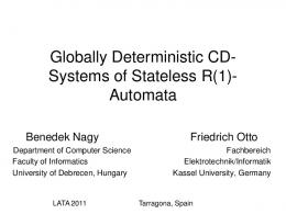
based on timing but not on event, for this reason this paper gives solutions and algorithms about how to express temporal information in systemC. 2.1. Time and SystemC One of the most important components in the SystemC library is the model of time. However, this is hidden to the programmer through the data type (class) sc_time. Therefore, in SystemC there is a minimum representable time quantum, called the time resolution. This can be set by the user. Note that this time resolution limits the maximum representable time, thus, any time value smaller than the time resolution will be rounded to zero. Today, SystemC can deal with the important notion of continuous time, not only discrete time. Our model exploit this approach in order to add continuous timing properties to SystemC models within delta-cycles. 2.2. A simple annotated FIFO model We start with a simple SystemC model: an implementation of FIFO with clocks. The model contains a First-In-First-Out buffer and two modules cooperating through the buffer: • the producer randomly generates data that is immediately sent to the consumer. • the consumer requests data at randomly-chosen points of time.
FIFO t_comm (write,t) (read,t)
Producer
Consumer
c_clock
p_clock FIFO: Timed FIFO write,t: w_event at t time. read,t: r_event at t time. FIGURE 1: A Timed FIFO
The necessary synchronization is performed by the FIFO that takes and delivers the generated data on demand.The two processes are triggered by two individual clocks: p_clock and c_clock. When a p_clock signal arrives, the producer starts producing and tries to write the product into
Third International Workshop on Verification and Evaluation of Computer and Communication Systems
3
Timed SystemC Waiting-State Automata
the buffer. Similarly, the c_clock signals control the consumer. The two clocks are independent, hence the producing and the consuming can be at different paces. Modeling is usually done with the perspective of performing analysis. Modeling for analysis requires building a model of the system and of the environment. In the context of real time systems the environment includes time properties and constraints. However, this model (the FIFO model) is deprived of temporal annotation, e.g when a producer starts producing and writing the product into the buffer and for how much time? besides there is no information about the duration of each event like w_event or r_event, about communication delays and the execution time. As a result the satisfaction of real time constraints cannot be verified. Modeling the time environment of systems means imposing constraints on time spent in transitions, in communications and also in all other implicitly defined activities. To overcome these limitations, we annotate the FIFO model with time information, so that we eliminate ambiguity about time execution. We take into account the synchronization between the two processes producer/consumer when releasing/filling buffer. It is not only the occurrence of an event that determines which process will be executed but also the time at which this event occurs, i.e the consumer can not start to read before the consumer has finished to write. We have two possible execution models, if the execution model is a sequential model, the time annotations are ordered, if the execution model is a concurrent model, we introduce time annotations as partially ordered. 2.3. Events and time SystemC is a modeling language based on C++ that is intended to enable system level design in response to the need of a very fast executable specification to validate and verify system concepts [7]. It provides structural description features including modules and ports that can be used in systems design. In addition, there exist different data types to enable modeling hardware systems, processes to express concurrency, channels, interfaces, and events to enable communication and synchronization between modules or processes. Despite of the diversity in syntax, SystemC is essentially an event-driven model and all communications in SystemC models are implemented using events and the associated wait/notify mechanism. The only possible action on an event is to trigger it. This is done with the notify function. A SystemC event is the result of such a notification, and has no value and no duration, but only happens at a single point in time and possibly triggers one or several processes. For instance, the FIFO module is actually defined as a channel sc_channel, and the mutual access to the buffer is implemented through the two events r_event and w_event. SystemC events can be roughly classified into the following three sorts: User-defined events These are events defined by SystemC programmers in source code. For instance, the w_event and the r_event. Such events are usually triggered by the command notify; Channel events These are pre-defined SystemC events and they are triggered when something occurs on channels. For instance, an event denoting the arrival of a new value will be triggered whenever some value is written to a sc_buffer channel. Channel events at different types of channels have different semantics; Clock events Clock signals are also seen as events and they are usually defined as sc_clock’s in the SystemC main program. SystemC core engine is in charge of generating sc_clock events at proper time. We never notify a clock event in the program. We shall not distinguish between the first two sorts of events since both of them can be dynamically notified. Clock events are rather seen as the input events of SystemC models. In fact, we prefer not considering any pre-defined channels or signals in our modeling, but rather taking into account their event-driven implementation.
Third International Workshop on Verification and Evaluation of Computer and Communication Systems
4
Timed SystemC Waiting-State Automata
An sc_event can be notified using immediate or timed notification. Immediate notification of e is achieved with e.notify();. The statement e.notify(t); triggers the event e at least at t time of simulated time (it overrides any previous timed notification that did not yet occur). A set of timing constraints is generated for each occurrence of an event or exactly when a transition is triggered. The above procedure formalize the concept of annotation or modeling time for high level synthesis: current_time = 0; while ( S i m u l a t i o n i s not achieved ) { w a i t t i l l t h e ev ent E oc c ur s ; c u r r e n t _ t i m e = g e t t h e time o f t h e ev ent E ; executes t h e process ; annotates t h e t r a n s i t i o n w i t h t h e c u r r e n t time , and t h e e x e c u t i o n time ( d u r a t i o n ) o f t h e t r a n s i t i o n } 2.4. SystemC simulator Most HDLs, VHDL for example, use a simulation kernel. The purpose of the kernel is to ensure that parallel activities (concurrency) are correctly modeled. The behavior of the simulation should not depend on the order in which the processes are executed at each step in simulation time. The SystemC simulation kernel introduces the notion of delta cycles. A delta cycle consists of an evaluation phase and an update phase. This is typically used for modeling primitive channels that cannot change instantaneously. By separating the two phases of evaluation and update, it is possible to guarantee deterministic behaviors. Here is a brief description of a delta-cycle: a delta-cycle starts with a non-empty runnable process table. The scheduler executes these processes one by one, in a pre-defined order; every runnable processes executes until it ends or it is pended again (by a wait command for instance); if any immediate event (e.g. the w_event generated by the producer process in the FIFO example) is notified during the execution of runnable processes, it will add processes that are currently sensitive to this event into the runnable process table; delta-events and timed events that are generated during the execution of a process are stored in other tables. The process table is emptied when all runnable processes are executed and the procedure of executing all the runnable processes is called an evaluation phase. The scheduler then checks those delta-events notified in the evaluation phase: if there are processes that are sensitive to these events, then add them into the process table. This procedure is called a delta notification phase. If the process table is non-empty, the scheduler enters the next delta-cycle and executes the evaluation phase again; otherwise, it checks the timed events notified in the evaluation phase and adds processes that sensitive to these timed events into the process table. This is called a timed notification phase. The scheduler then advances the simulation clock and enters the next delta-cycle. SystemC simulation kernel contains a scheduler to determine the order of execution of processes within the design based on the event sensitivity of the processes and the event notifications which occur. It supports both software and hardware-oriented modeling. 3. EXTENDING SYSTEMC WAITING STATE AUTOMATA WITH TIME Unlike some other formal models such Petri nets [5] and Finite-State Automata that are used to model concurrent distributed systems, the WSA [2] is a formal model for verifying SystemC components that is based on the waiting states of processes within a delta cycle and that conforms to the SystemC scheduler up to delta cycle. The basic idea of Waiting-State Automata’s is to consider only the states where processes are hung up, i.e. waiting for some events. In fact, a delta-cycle always starts from a state where all the processes are hung up and the whole cycle can be seen as a sequence of transitions between these waiting states. A main drawback of this model is that all information about time properties get lost. First, refining SystemC code with
Third International Workshop on Verification and Evaluation of Computer and Communication Systems
5
Timed SystemC Waiting-State Automata
respect to the delta-cycle semantics abstract delta-cycles to untimed atomic transitions. Secondly, during SystemC simulation, precise information about execution time are not available. To overcome those limitations, we annotate each transition with some additional information about time properties and time constraints. More precisely, transitions are timed; ie. a transition can only be activated if a given time condition is verified and it also defines how long it takes to be executed. Let us illustrate this on the FIFO example and consider the two small automata for the processes of the producer and the consumer. Figure 2 shows both automata annotated with times. For
,t
2 r
w
,
2
,
2
{p_clock}, (num_elem k dkτ . As the transition predicates (i.e., guard conditions) in timed waiting-state automata are defined over the timers and system variables, the composition should ensure that these predicates of component automata are properly translated in the composed automaton. In particular, we must replace all the occurrence of a transition starting time and duration from component automata, with the values t and d recently presented. We consider a timed automaton as deterministic when it does not contain any non-deterministic transition. In the untimed case a deterministic transition has a single start state and from each state, given the next sc_event, the next state is uniquely determined. We want similar criterion for determinism for the timed automata: given an extended state and the next input sc_event along with its time of occurence, the extended state after the next transition should be uniquely determined.
Algorithm 1 (Symbolic composition) Given two timed SystemC waiting-state automata A(V ) = (S; E; T ; Υ; D) and A′ (V ) = (S ′ ; E ′ ; T ′ ; Υ′ ; D′ ), over a set V of variables, the combination of the two timed SystemC waiting-state automata is still a timed SystemC waiting-state automaton S (S × S ′ ; E E ′ ; T ′′ ; Υ′′ ; D′′ ) written as A(V ) × A′ (V ) where T ′′ is the smallest set of transitions, Υ′′ the associated set of the starting times and D′′ is the corresponding set of durations, Π(s; ein ; p; t; eout ; f ; d; s′ ) is the set of times of Υ′′ and D′′ associated to a transition in T × T ′ and Mt a morphism that maps starting times in Υ × Υ′ to Υ′′ , Md a morphism that maps duration times in D × D′ to D′′ such that: S • Π(s1 ; ein ; p; t; eout ; f ; d; s2 ) := {t∗ , d∗ } Π(s1 ; ein ; p; t; eout ; f ; d; s2 ) and ′
ein ,Mt (p),Md (p),t∗
′
ein ,p,t
(s1 , s1 ) −−−−−−−− −−−−→ (s2 , s1 ) ∈ T ′′ for every transition s1 −−−−−→ s2 ∈ T and for ′ eout ,f ,d∗
eout ,f,d
Third International Workshop on Verification and Evaluation of Computer and Communication Systems
7
Timed SystemC Waiting-State Automata ′
′
′
e
′
′
,p ,t
′
′
every state s1 ∈ S ′ such that for every transition s1 −− −in −−−−−→ s2 ∈ T ′ , either ein * ein or ′ ′ eout ,f ′ ,d′ ,s2
′
p;p; ′ ′ ′ ′ • Π(s1 ; ein ; p′ ; t′ ; eout ; f ; d′ ; s2 ) ′
{t∗ , d∗ }
:=
′ ein ,Mt (p′ ),Md (p′ ),t∗
′
S
′
′
′
′
Π(s1 ; ein ; p′ ; t′ ; eout ; f ; d′ ; s2 ) ′
′ ein ,p′ ,t′
and
′
(s1 , s1 ) −−−−−′−−−−−−−−→ (s1 , s2 ) ∈ T ′′ for every transition s1 −− −−−−→ s2 ∈ T ′ and ′ eout ,f ′ ,d∗
eout ,f ′ ,d′
ein ,p,t
′
for every state s1 ∈ S such that for every transition s1 −−−−−→ s2 ∈ T, either ein * ein or eout ,f,d
′
p ; p; • Π(s1 ; ein ; p; t; eout ; f ; d; s2 ) ′ ′ ′ ′ ′ ′ ′ Π(s1 ; ein ; p ; t ; eout ; f ; d ; s2 ) ′
(s1 , s1 ) ein ,p,t
ein
S
′
e
,Mt (p∧p′ ),Md (p∧p′ ),t∗
−−−−−in −−− −−−−− −−−−−→ S−− ′ ′ eout
eout ,f ◦f
′
′
e
S {t∗ , d∗ }S Π(s1 ; ein ; p; t; eout ; f ; d; s2 ) ′ ′ ′ ′ ′ ′ ′ {t∗ , d∗ } Π(s1 ; ein ; p; t ; eout ; f ; d ; s2 )
:= := ,d∗
′
′
(s2 , s2 )
∈
and and
T ′′ , for every pair of transitions
′
,p ,t
′
in s1 −−−−−→ s2 ∈ T and s1 −− −−−′−→ s2 ∈ T ′ . ′ ′
eout ,f,d
eout ,f ,d
• According to the transition (s1 ; ein ; p; tss21 ; eout ; f ; dss21 ; s2 ), the morphism Mt maps the starting t to the min of transition starting times defined in Π(s1 ; ein ; p; t; eout ; f ; d; s2 ) M (t) → mint∗ ∈Π(s1 ,ein ,p,t,eout ,f,d,s2 ) t∗ • According to the transition (s1 ; ein ; p; tss21 ; eout ; f ; dss21 ; s2 ), the morphism Md maps the the duration d to the sum of durations defined in Π(s1 ; ein ; p; t; eout ; f ; d; s2 ) X d∗ . M (d) → d ≥ d∗ ∈Π(s1 ,ein ,p,t,eout ,f,d,s2 )
Algorithm 2 (Symbolic reduction) Given a timed SystemC minimal-step waiting-state automaton A(V ) = (S; E; T ; Υ; D), where T has reducible transitions, let T0 := T , Υ0 := Υ, D0 := D, let Tremove ; Tnew := {}; Υremove ;Υnew ; Dremove ; Dnew := {}. The following steps define an algorithm to remove all the reducible transitions: 1. for every its contractum t3 , where t1 , t2S∈ T0 , let: Tremove := S reducible pair (t1 ; t2 ) and S Tremove {t1 } and Tnew := Tnew {tS 3 }; Υremove := Υremove { the starting times { the starting time associated to associated to t and t }; Υ := Υ 1 2 new new S S t3 }; Dremove := Dremove { the durations associated to t1 and t2 }; Dnew := Dnew { the durations associated to t3 }; replaces the starting time and the duration associated to the removed transitions t1 and t2 that appear in all the pre-conditions and post-conditions defined in T0 with the new couple of time associated to the transition t3 . 2. repeat the above step until all reducible pairs in T0 have been manipulated; S 3. Let T0 := S (T0 /Tremove ) ∪ Tnew , let Υ0 := (Υ0 /Υremove ) Υnew , let D0 := (D0 /Dremove ) Dnew ; 4. let Tremove ; Tnew ; Υremove ; Dremove ; Υnew := {} ; Dnew := {}. 5. if there are still reducible pairs in T0 , go to the step 1 and repeat the above procedure; otherwise, let T ′ := T0 ; Υ′ := Υ0 , D′ := D0 . The reduced automaton is (S; E; T ′ ; Υ′ ; D′ ). 4. EXTENDING TIMED SYSTEMC WAITING STATE AUTOMATA WITH COUNTERS In the previous section, transitions were annotated with temporal information: the starting time and the delay, which makes the automaton a nice framework for the verification of reactive systems. We add a new timescale to the whole system within a delta cycle considering only moments when a process get into and get out of a waiting state. Moreover we can extend in a nice way the previous model with counters that counts the number of times a transition has been activated. Combining the both information, the time at which a
Third International Workshop on Verification and Evaluation of Computer and Communication Systems
8
Timed SystemC Waiting-State Automata
transition is activated, the execution of the transition as well as the number of time a transition has been actived allow to infer precise information about the system time execution; i.e if we take each process separately and we study how many times it gets into a waiting state and for how much duration, we can compute the lower bound of its execution time. When we compose processes automata together to get a bigger one using the same parameters time and counters, we obtain more information about the model and its execution time and consequently, we are able to verify additional relevant properties and infer new time constraints.
4.1. The automata for the producer and the consumer annotated with time and counters Again, let us look at the FIFO example and consider the two small automata’s for the processes of the producer and the consumer. In this section we will try to define new relations between both times and counters considering in addition to that the total execution time. We have usually 3 the same definitions for our parameters, e.g γw counts the times of executing the transition from 1 p_wait_clk to p_wait_c, and tr represents the time the consumer starts reading. Usually we have
,t
g 2r
2 r
g 2w
2
,
dr
2
{p_clock}, (num_elem k tτ . As the transition predicates (i.e., k dτ and γ = guard conditions) in the extended timed waiting-state automata are defined over the timers, couters and system variables, the composition should ensure that these predicates of component automata are properly translated in the composed automaton. In particular, we must replace all the occurrence of a transition starting time, duration and couter from component automata, with the values t, d and γ recently presented.
Symbolic composition Given two timed SystemC waiting-state automata A(V ) = (S; E; T ; Υ; D; Γ) and A′ (V ) = (S ′ ; E ′ ; T ′ ; Υ′ ; D′ ; Γ′ ), over the same set V of variables, the combination S of the two SystemC waiting state automata is still a SystemC waiting-state automaton (S ×S ′ ; E E ′ ; T ′′ ; Υ′′ ; D′′ ; Γ′′ ) written as A(V )×A′ (V ) where T ′′ is the smallest set of transitions, Υ′′ is the associated set of the starting times, D′′ is the corresponding set of durations and Γ′′ is the associated set of counters, Π(s; ein ; p; t; eout ; f ; d; s′ ; γ) is the set of times and counters of Υ′′ , D′′ and Γ′′ associated to a transition in T × T ′ and . Mc a morphism that maps counters in Γ × Γ′ to Γ′′ , Mt a morphism that maps times in Υ × Υ′ to Υ′′ and Md a morphism that maps times in D × D′ to D” such that: S • Π(s1 ; ein ; p; t; γ; eout ; f ; d; s2 ) := {t∗ , d∗ , γ ∗ } Π(s1 ; ein ; p; t; γ; eout ; f ; d; s2 ) and ′
ein ,Mt (p),Mc (p),Md (p),t∗ ,γ ∗
ein ,p,t,γ
′
(s1 , s1 ) −−−−−−−−−−−′−−−−−−−−→ (s2 , s1 ) ∈ T ′′ for every transition s1 −−−−−→ s2 ∈ T eout ,f,d
eout ,f ,d∗
′
′
′
′
′
ein ,p ,t ,γ
′ ′
and for every state s1 ∈ S ′ such that for every transition s1 −− −−−−−−→ s2 ∈ T ′ , either ′ ′ eout ,f ′ ,d′ ,s2
′
′
ein * ein or p ; p ; ′ ′ ′ ′ • Π(s1 ; ein ; p′ ; t′ ; γ ′ ; eout ; f ; d′ ; s2 ) ′
:=
′ ein ,Mt (p′ ),Mc (p′ ),Md (p′ ),t∗ ,γ ∗
{t∗ , d∗ , γ ∗ } ′
S
′
Π(s1 ;
′
′
′
′
ein ; p′ ; t′ ; γ ; eout ; f ; d′ ; s2 ) and ′
′ ein ,p′ ,t′ ,γ ′
′
(s1 , s1 ) −−−−−−−−− −−−−−−−−−−−→ (s1 , s2 ) ∈ T ” for every transition s1 −−′−−−−−→ s2 ∈ T ′ ′ (eout
,f ′ ,d∗)
eout
,f ′ ,d′
Third International Workshop on Verification and Evaluation of Computer and Communication Systems
10
Timed SystemC Waiting-State Automata ein ,p,t,γ
′
and for every state s1 ∈ S such that for every transition s1 −−−−−→ s2 ∈ T, either ein * ein eout ,f,d
′
or p ; p; • Π(s1 ; ein ; p; t; γ; eout ; f ; d; s2 ) ′ ′ ′ ′ ′ ′ ′ ′ Π(s1 ; ein ; p ; t ; γ eout ; f ; d ; s2 ) ′
ein
S
′
e
S {t∗ , d∗ , γ ∗ }S Π(s1 ; ein ; p; t; γ; eout ; f ; d; s2 ) ′ ′ ′ ′ ′ ′ ′ ′ {t∗ , d∗ , γ ∗ } Π(s1 ; ein ; p; t ; γ eout ; f ; d ; s2 )
:= :=
,Mt (p∧p′ ),Mc (p∧p′ ),Md (p∧p′ ),t∗ ,γ ∗
and and
′
in (s1 , s1 ) −−−−−− −−−−−−S −−− −−−−′−−−−−−−−−−→ (s2 , s2 ) ∈ T ”, for every pair of transitions ′
ein ,p,t,γ
eout
eout ,f ◦f ,d∗ ′
′
e
′
′
,p ,t ,γ
′
′
′
in s1 −−−−−→ s2 ∈ T and s1 −− −−−− −→ s2 ∈ T . ′ ′ ′
eout ,f,d
eout ,f ,d
• According to the transition (s1 ; ein ; p; tss21 ; eout ; f ; dss21 ; s2 ; γss12 ), the morphism Mt maps the starting t to the min of transition starting times defined in Π(s1 ; ein ; p; t; eout ; f ; d; s2 ; γ) M (t) → mint∗ ∈Π(s1 ,ein ,p,tss2 ,eout ,f,dss2 ,s2 ,γss2 ) t∗ 1
1
1
• The morphism Md maps the the duration d to the sum of durations defined in Π(s1 ; ein ; p; t; eout ; f ; d; s2 ; γ) X M (d) → d ≥ d∗ . s
s
s
d∗ ∈Π(s1 ,ein ,p,ts21 ,eout ,f,ds21 ,s2 ,γs12 )
• The morphism Mc maps the counters γ to the sum of counters defined in Π(s1 ; ein ; p; t; eout ; f ; d; s2 ; γ) X M (γ) → γ∗. s
s
s
γ ∗ ∈Π(s1 ,ein ,p,ts21 ,eout ,f,ds21 ,s2 ,γs12 )
Symbolic reduction Given a SystemC minimal-step waiting-state automaton A(V ) = (S; E; T ; Υ; D; Γ), where T has reducible transitions, let T0 := T ,D0 := D,Υ0 := Υ, Γ0 := Γ, let Tremove ; Tnew ; Dremove ; Υremove ; Γremove ; Dnew := {};Υnew := {}; Γnew := {}. The following steps define an algorithm of removing the reducible transitions: 1. For every S its contractum t3 , whereSt1 , t2 ∈ T0 , let: Tremove := S reducible pair (t1 ; t2 ) and Tremove {t1 } and Tnew :=STnew {t3 }; Γremove = Γremove { the counters associated S to t1 and t2 };Γnew = Γnew { the counters associated S to t3 }; Υremove = Υremove { the to t3 }; starting times associated to t1 and t2 }; Υnew = Υnew { the starting time associated S S Dremove = Dremove {the durations associated to t1 and t2 }; Dnew = Dnew { the durations associated to t3 }; replaces the starting time, the duration and the counters associated to the removed transitions t1 and t2 that appear in all the pre-conditions and post-conditions defined in T0 with the new values associated to starting time, duration and the counter associated to the transition t3 . 2. Repeat the above step until all reducible pairs in T _0 have been manipulated; S 3. Let T0 := S(T0 /Tremove ) ∪ Tnew , let Υ0 S := (Υ0 /Υremove ) Υnew , let D0 := (D0 /Dremove ) Dnew and let Γ0 := (Γ0 /Γremove ) Γnew 4. let Tremove ; Tnew ;Υremove ; Dremove ; Γremove ; Υnew := {}; Dnew := {} and Γnew := {}. 5. If there are still reducible pairs in T0 , go to the step 1 and repeat the above procedure; ′ ′ otherwise, let T ′ := T 0; Υ := Υ0 ; D := D0 and Γ′ := Γ0 . The reduced automaton is (S; E; T ′ ; Υ′ ; D′ ; Γ′ ). 5. CONCLUSION Verification of reactive systems, critical systems or embedded systems is a very important issue today. The increasing complexity requires more design efforts and choosing the right architecture to garantee system performance and realibility requires large design space exploration. In this paper, we propose a new formal model to verify real-time systems described in a high level langage: SystemC. This model provides the capacity to verify timed SystemC designs, to infer or
Third International Workshop on Verification and Evaluation of Computer and Communication Systems
11
Timed SystemC Waiting-State Automata
verify time constraints as well as to estimate partial or global system execution time, at the level of delta cycles. The process of the verification of timed SystemC design is clear; we first translate SystemC processes into timed SystemC waiting-state automata. We then combine those automata together. During all the combination, we may infer affine relations regarding transition counts as well as the time at which transitions can be activated. We finally reduce the resulting automaton so that the final automata recognize the abstraction of the whole system at the level of deltacycles. Timed SystemC waiting state automata may also be a valuable representation for timed co-simulation [9,10]. REFERENCES [1] K. Richter, M. Jersak, R. Ernst, A formal approach to MpSoC performance verification, Computer, April 2003. [2] Yu Zhang, Franck Védrine, Bruno Monsuez, SystemC Waiting-State Automata, 2008 http://www.bcs.org/upload/pdf/ewic_ve07_s2paper2.pdf [3] F. Balarin, L. Lavagno, P. Murthy, A. SanGiovanni-Vicentelli, Scheduling for embedded realtime systems, IEEE Design & Test of Computers, January-March 1998. [4] SystemC homepage. http://www.systemc.org. [5] J. L. Peterson, Petri Nets, 1977 ˜ http://www.cs.olemiss.edu/dwilkins/Seminar/S05/PetersonPetri.pdf. [6] Richard M.Fujimoto, Time Management in the High Level Architecture, 1998 http://www.cc.gatech.edu/computing/pads/PAPERS/Time_mgmt_High_Level_Arch.ps. [7] H.Posadas, F.Herrera, P.Sànchez, E.Villar & F.Blasco, System-Level Performance Analysis in SystemC, 2004 http://date.eda-online.co.uk/proceedings/papers/2004/date04/pdffiles/04b_2.pdf. [8] S. Yoo, G. Nicolescu, L. Gauthier, A. Jarraya, Automatic generation of fast timed simulation models for operating systems in SoC design, Proc. of DATE, IEEE, 2002. [9] J.Y. Lee, I. Park, Timed Compiled-Code Simulation of Embedded Software for Performance Analysis of SoC [10] E. Clarke, O. Grumberg, D. Peled, Model-Checking, The MIT Press, Cambridge, Massachusetts, 1999. [11] Ph. Schnoebelen, B. Bérard, M. Bidoit, F. Laroussinie, A. Petit, Systems and Software Verification - Model-Checking Techniques and Tools, Springer, 2001. [12] Amjed Gawanmeh, Ali Habibi, Sofène Tahar, Enabling SystemC Verification using Abstract State Machines, 2004 http://hvg.ece.concordia.ca/Publications/TECH_REP/SYSC_TR04/SYSC_TR04.pdf. A. THE TIMED SYSTEMC WAITING STATE OF THE FIFO MODEL
Third International Workshop on Verification and Evaluation of Computer and Communication Systems
12
{ }, id, { d
3 r 2
2
2
+dw}
{p_clock }, (num_elem0}, t r
2
{w_event, r_event }, {inc & dec}, { d r +d
2 3 w
{r_event, c_clock }, ( num_elem>0),{ min(t w ,t r )} }
+d
2 w
}
2 w
c_wait_clk , p_wait_c
3 r
3 r
1
{ }, id, d
2 r
2
}
1 r 1 r
3
1 {w_event }, inc , d w
{r_event }, dec, d
{w_event }, ( ), t
{ }, id,
d 3r
+
2 dw
1 {r_event }, ( ), { t w }
1 r
2 w
{c_clock} ,(num_elem=0), t r
2
{r_event }, dec & inc, d
{c_clock }, (num_elem