Two-Microphone Source Separation Algorithm Based on ... - CiteSeerX

TWO-MICROPHONE SOURCE SEPARATION ALGORITHM BASED ON STATISTICAL MODELING OF ANGLE DISTRIBUTIONS Chanwoo Kim 1 , Charbel Khawand 2 and Richard M. Stern 3 Windows Phone Division Microsoft Corporation1,2 , Redmond WA 98052 USA Department of Electrical and Computer Engineering Carnegie Mellon University3, Pittsburgh PA 15213 USA ABSTRACT In this paper we present a novel two-microphone sound source separation algorithm, which selects speech from the target speaker while suppressing signals from interfering sources. In this algorithm, which is refered to as SMAD-CW, we first estimate the direction of sound sources for each time-frequency bin using phase differences in the spectral domain. For each frame we assume that the angle distribution is a mixture of two distributions, one from the target and the other from the dominant noise source. For each mixture component we use the von Mises distribution, which is a close approximation to the wrapped normal distribution. The expectation-maximization (EM) algorithm is employed to obtain parameters of this mixture distribution. Using this statistical model, we perform maximum a posteriori (MAP) hypothesis testing in order to obtain appropriate binary masks. We demonstrate that the algorithm described in this paper provides speech recognition accuracy that is significantly better than that obtained using conventional approaches. Index Terms— Robust speech recognition, signal separation, interaural time difference, statistical modeling, binaural hearing, von Mises distribution 1. INTRODUCTION Speech recognition systems have significantly improved in recent years, and they have been used in many applications. Even though we can obtain high speech recognition accuracy in clean environments using state-of-the-art speech recognition systems, performance seriously degrades in noisy environments. Thus, noise robustness remains a critical issue for speech recognition systems that are used for real consumer products in difficult acoustical environments. Many algorithms have been developed to address these problems, and a number of them have proved to be of significant value in reducing the impact stationary noise. Nevertheless, improvement in non-stationary noise remains elusive. An alternative approach is signal separation based on analysis of differences in arrival time (e.g. [1, 2]). It is well known that the human binaural system is remarkable in its ability to separate speech from interfering sources (e.g. [3]). Motivated by these observations, many models and algorithms have been developed using interaural time differences (ITDs), interaural intensity difference (IIDs), interaural phase differences (IPDs), and other cues (e.g. [1, 2, 4]). IPD and ITD have been extensively This research was supported by the Microsoft Corporation and by the NSF (Grant IIS-I0916918). The authors are grateful to Prof. Bhiksha Raj and Kshitiz Kumar for many useful discussions.

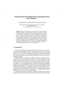
used in binaural processing because this information can be easily obtained by spectral analysis (e.g. [5]). In the present approach, we use statistical modeling of angle distributions with channel weighting (SMAD-CW) instead of a fixed threshold to determine which signal components belong to the target signal and which components are part of the background noise. 2. STRUCTURE OF THE SMAD-CW ALGORITHM The CWAD-CW algorithm crudely emulates selected aspects of human binaural processing and is summarized by the block diagram of Fig. 1. While the description below assumes a sampling rate of 16 kHz and 4 cm between the two microphones, the algorithm is easily modified to accommodate other sampling frequencies and microphone separations. In our discussion we assume that the location of the target source is known a priori, and lies along the perpendicular bisector of the line between the two microphones. Short-time Fourier transforms (STFTs) are performed on the signals from the left and right microphonesusing Hamming windows of duration 75 ms, 37.5 ms between successive frames, and a DFT size of 2048. The choice of a rather long window has been discussed previously (e.g. [5]). For each time-frequency bin, the direction of the sound source is estimated indirectly by comparing the phase information from the two microphones. Either the angle or ITD information is used as a statistic to represent the direction of the sound source, as described in Sec. 3.1. Most conventional algorithms using a pair of microphones compare the signal components in each time-frequency bin to a threshold angle or ITD to determine whether the signal component in each time-frequency bin is likely to originate from the target or a noise source (e.g. [1, 5]). The SMAD-CW algorithm, in contrast, models the angle distribution for each frame as a mixture of two Von Mises distributions; one from the target and the other from the noise source. The von Mises distribution, which is a close approximation to the wrapped normal distribution, is used rather than the wellknown Gaussian distribution because the angle is limited between − π2 and π2 . Parameters of the distribution are estimated using the expectation-maximization (EM) algorithm, as described in Sec. 3.2. After obtaining parameters of the angle distribution, we perform maximum a posteriori (MAP) testing on each time-frequency bin. From these results binary masks are constructed based on whether a specific time-frequency bin is likely to be occupied by the target distribution or the noise distribution. Hence, SMAD-CW employs a soft decision approach based on statistical hypothesis testing. To obtain better speech recognition accuracy in noisy environments, we apply the gammatone channel weighting approach intro-

xL [ n ]

STFT

X L [ m, e jωk )

X R [m, e jωk )

xR [ n ]

Angle Estimation From Phase

θ [m, k ]

Mixture Distribution Estimation


[m ]

µ [ m, k ]

Gammatone Channel Weighting

µ s [m, k ]

Hypothesis Testing

H1 > η [ m] g [ m, k ] < H0

STFT Binary Mask Construction

Applying Masks

Y [ m , e jω k )

STIFT and OLA

y[n ]

X A[m, e jωk )

Fig. 1. The block diagram of a sound source separation system based on the Statistical Modeling of Angles and likelihood Ratio Testing (SMAD) algorithm. duced in [5] rather than directly applying the binary mask. In gamrefer to this limited ITD estimate as τ˜[m, k]. The estimated angle matone channel weighting, the ratio of power after applying the biθ[m, k] is obtained from τ˜[m, k] using nary mask to the original power is obtained for each channel, which   cair τ˜[m, k] is subsequently used to modify the original input spectrum, as de(4) θ[m, k] = asin scribed in Sec. 3.4. Finally, the time domain signal is obtained by fs d the overlap-add (OLA) method. The SWAD algorithm with channel weighting is referred to as SMAD-CW. Each component of the 3.2. Statistical modeling of the angle distribution SWAD-CW algorithm is described in further detail in Sec. 3. For each frame, the distribution of estimated angles θ[m, k] is modeled as a mixture of the target and the noise distributions: 3. COMPONENTS OF SMAD-CW PROCESSING fT (θ|M[m]) = c0 [m]f0 (θ|µ0 [m], κ0 [m]) 3.1. Estimation of the angle for each frequency index +c1 [m]f1 (θ|µ1 [m], κ1 [m]) (5) In each frame, the phase differences between the left and right spectra are used to estimate the intermicrophone time difference (ITD), and subsequently the angle of the sound source, as described previously in [5] and elsewhere. Let XL [m, ejωk ) and XR [m, ejωk ) represent the STFT of the signals from the left and right microphones, respectively, where wk = 2πk/N and N is the FFT size. We refer to τ [m, k] as the ITD at frame index m and frequency index k. We obtain the relationship φ[m, k] , ∠XR [m, ejωk ) − ∠XL [m, ejωk ) = wk τ [m, k] + 2πl (1) where l is an integer chosen such that   if |φ[m, k]| ≤ π φ[m, k], wk τ [m, k] = φ[m, k] − 2π, if φ[m, k] ≥ π  φ[m, k] + 2π, if φ[m, k] < −π

(2)

(In these discussions we consider only values of the frequency index k that correspond to positive frequency components, 0 ≤ k ≤ π/2.) If a sound source is located along a line of angle θ[m, k] with respect to the perpendicular bisector to the line between the microphones, geometric considerations determine the ITD τ [m, k] to be τ [m, k] =

d sin(θ[m, k]) fs cair

(3)

where cair is the speed of sound in air (assumed to be 340 m/s in our work) and fs is the sampling rate. While in principle |τ [m, k]| cannot be larger than τmax = fs d/cair from Eq. (3), in real environments |τ [m, k]| may be larger than τmax because of approximations in the assumptions that were made if the ITD is estimated directly from Eq. (2). For this reason we limit τ [m, k] to lie between between −τmax and τmax and we

where c1 [m] and c0 [m] are the mixture coefficients, and M[m] is the set of parameters of the mixture distribution. In this section we use the subscript 0 to represent the noise and the subscript 1 to represent the target. Specifically,  M[m] = c1 [m], µ0 [m], µ1 [m], κ0 [m], κ1 [m] (6) fT (θ|µ1 [m], κ1 [m]) and fN (θ|µ0 [m], κ0 [m]) are given as follows: f0 (θ|µ0 [m], κ0 [m]) = f1 (θ|µ1 [m], κ1 [m]) =

exp(κ0 [m] cos(2θ − µ0 [m])) πI0 (κ0 [m]) exp(κ1 [m] cos(2θ − µ1 [m])) πI0 (κ1 [m])

(7a) (7b)

The coefficient c0 [m] follows directly from the constraint c0 [m] + c1 [m] = 1. Since the parameters M[m] cannot be directly estimated in closed form, we obtain them using the EM algorithm. We impose the following constraints in parameter estimation: 0 ≤ |µ1 [m]| ≤ θ0 π θ0 ≤ |µ0 [m]| ≤ 2 θ0 ≤ |µ1 [m] − µ0 [m]|

(8a) (8b) (8c)

where θ0 is a fixed angle that equals 15π/180 in the present work. This constraint is applied both in the initial stage and the update stage explained below. Without this constraint µ0 [m] and κ0 [m] may converge to the target mixture or µ1 [m] and κ1 [m] may converge to the interference mixture, which would be problematical. Initial parameter estimation: To obtain the initial parameters of M[m], we consider the following two partitions of the frequency index k  K0 [m] = k θ[m, k] ≥ θ0 , 0 ≤ k ≤ N/2 (9a)  K1 [m] = k θ[m, k] < θ0 , 0 ≤ k ≤ N/2 (9b)

In this initial step, we assume that if the frequency index k belongs to K1 [m], then this time-frequency bin is dominated by the target; therwise, we assume that it is dominated by the noise. This initial step is similar to approaches using a fixed threshold. Consider a variable z[m, k] which is defined as follows: z[m, k] = ej2θ[m,k]

(10)

(0) z¯j [m]:

Let us define the weighted average PN/2 (0) k=0 ρ[m, k]I (θ[m, k] ∈ Kj ) z[m, k] z¯j [m] = PN/2 k=0 ρ[m, k]I (θ[m, k] ∈ Kj )

(11)

where I is the indicator function. The following equations are used in analogy to Eq. (17). P k∈Kj ρ[m, k] (0) cj [m] = PN/2 (12a) k=0 ρ[m, k]   (0) (0) µj [m] = Arg z¯j [m] (12b) (0)

I1 (κj [m])

(0) I0 (κj [m])

(0)

= |¯ zj [m]|

(12c)

where I0 (κj ) and I1 (κj ) are modified Bessel functions of the zeroth and first order. Parameter update: The E-step is given as follows: ˜ Q(M[m], M(t) [m]) N/2

=

X

k=0

h

 i ρ[m, k]E log fT θ[m, k], s[m, k]|θ[m, k], M(t) [m]

(13)

where ρ[m, k] is a weighting coefficient defined by ρ[m, k] = |XA [m, ejωk )|2 , and s[m, k] is the latent variable denoting whether the kth frequency element originates from the target source or the noise source. XA [m, ejωk ) is defined by: h i XA [m, ejωk ) = XL [m, ejωk ) + XR [m, ejωk ) /2 (14) Given the current estimated model M(t) [m], we define the condi(t) tional probability Tj [m, k] as follows: (t)

Tj [m, k]

=

P (s[m, k] = j|θ[m, k], M(t) [m]), (t)

=

cj fj (θ[m, k]|µj , κj ) (t) j=0 cj fj (θ[m, k]|µj , κj )

P1

Let us define the weighted mean of z¯(t) [m] as follows: PN/2 (t) (t) k=0 ρ[m, k]Tj [m, k]z[m, k] z¯j [m] = PN/2 (t) k=0 ρ[m, k]Tj [m, k]

(15)

(16)

Using Eqs. (15) and (16), it can be shown that the following update equations maximize Eq. (13): P N2 (t) (t+1) k=0 ρ[m, k]Tj [m, k] (17a) cj [m] = P N2 k=0 ρ[m, k]   (t+1) (t) µj [m] = Arg z¯j [m] (17b) (t+1)

[m])

(t+1)

[m])

I1 (κj

I0 (κj

(t)

= |¯ zj [m]|

(17c)

Assuming that the target speaker does not move rapidly with respect to the microphone, we apply the following smoothing to improve performance: µ ˜1 [m] = λµ1 [m − 1] + (1 − λ)µ1 [m] κ ˜ 1 [m] = λκ1 [m − 1] + (1 − λ)κ1 [m]

(18) (19)

with the forgetting factor λ equal to 0.95. The parameters µ ˜1 [m] and κ ˜ 1 [m] are used instead of µ1 [m] and κ1 [m] in subsequent iterations. This smoothing is not applied to the representation of the noise source. 3.3. Hypothesis Testing Using the obtained model M[m] and Eq. (7), we obtain the following MAP decision criterion: H1

g[m, k] > < η[m]

(20)

H0

where g[m, k] and η[m] are defined as follows: g[m, k] = κ1 [m] cos (2θ[m, k] − µ1 [m]) −κ0 [m] cos (2θ[m, k] − µ0 [m])   I0 (κ1 [m])c0 [m] η[m] = ln I0 (κ0 [m])c1 [m]

(21) (22)

Using Eq. (20) we construct a binary mask µ[m, k] for each frequency index k as follows: ( 1 if g[m, k] ≥ η[m] µ[m, k] = (23) 0 if g[m, k] < η[m] Processed spectra are obtained by applying the mask µ[m, k], and speech is resynthesized using the IFFT and OLA. This approach (without the channel weighting described in Sec. 3.4) is referred to as SMAD reconstruction. 3.4. Applying channel weighting To reduce the impact of discontinuities associated with binary masks, we obtain a weighting coefficient each channel. Each  for  j ωk of these channels is associated with Hl e , the frequency response of one of a set of gammatone filters, as specified in [6]. Let w[m, l] be the square root of the ratio of the output power to the input power for frame index m and channel index l: v 2  u P N −1 ωk ωk u 2 j j u k=0 XA [m, e )µ[m, k]Hl (e )  u w[m, l] = max  , δ 2 t  (24) P N2 −1 j ωk )H (ej ωk ) [m, e X A l k=0 where δ is a flooring coefficient that is set to 0.01 in the present implementation. Note that the channel weighting coefficient w[m, l] is somewhat different from the coefficient in our previous paper [5]. Using w[m, l], speech is resynthesized in the same fashion as in [5]. 4. EXPERIMENTAL RESULTS In this section we present experimental results using the SMAD-CW algorithm described in this paper. To evaluate the effectiveness of

= 0 ms)

RM1 (RT

60

Accuracy (100 − WER)

Accuracy (100 − WER)

60

80 60 40 20 0 0

5

10 15 SIR (dB)

20

Clean

RM1 (RT

= 100 ms)

60

100

Accuracy (100 − WER)

RM1 (RT 100

80 60 40 20 0 0

5

10 15 SIR (dB)

(a)

20

80 60 SMAD−CW SMAD PDCW ZCAE Single Mic

40 20 0 0

Clean

= 200 ms)

100

5

(b)

10 15 SIR (dB)

20

Clean

(c)

Fig. 2. Comparison of recognition accuracy for the DARPA RM database corrupted by an interfering speaker placed at 30◦ with respect to the perpendicular bisector to the line connecting the two microphones with three reverberation times: (a) 0 ms, (b) 100 ms, and (c) 200 ms. RM (Omni−Directional Noise) 100 Accuracy (100 − WER)

the statistical modeling of angle distributions and channel weighting, we compare performance of the SMAD-CW, SMAD, with the state-of-the art PDCW algorithm, as well as the baseline processing provided by the ZCAE algorithm [2] using binary masking. For ZCAE processing, we use zero-phase gammatone filter coefficients as described in [7]. Speech recognition experiments were performed using the reconstructed signals obtained as in Sec. 3 in conjunction with conventional MFCC features implemented as in sphinx fe in sphinxbase 0.4.1. For acoustic model training we used SphinxTrain 1.0, and decoding was performed suing the CMU Sphinx 3.8. We used subsets of 1600 utterances and 600 utterances, respectively, from the DARPA Resource Management (RM1) database for training and testing. A bigram language model was used in all experiments. In all experiments, we used feature vectors of length of 39 including delta and delta-delta features. We assumed that the distance between two microphones is 4 cm. The first set of experiments was conducted using simulated reverberant environments in which the target speaker is masked by a single interfering speaker. We assumed that the target is located along the perpendicular bisector of the line between two microphones, so θT = 0◦ . We assume that the interfering source is located at θI = 30◦ . Reverberation simulations were accomplished using the Room Impulse Response open source software package [8] based on the image method [9]. In the experiments in this section, we assumed room dimensions of 5 × 4 × 3 m, with microphones that are located at the center of the room. Both the target and interfering sources are 1.5 m away from the microphone. For the fixed-ITDthreshold systems PDCW and ZCAE, we used the threshold angle θT H = 15◦ . As shown in Fig. 2(a), in the absence of reverberation at 0-dB signal-to-interference ratio (SIR), the fixed-ITD-threshold systems PDCW and ZCAE and the SMAD-CW system provide comparable performance. In contrast, the SMAD-CW system provides substantially better performance than the PDCW signal separation system in the presence of reverberation. In the second set of experiments, we added noise recorded in real environments with real two-microphone hardware in locations such as a public market, a food court, a city street and a bus stop. These real noises were digitally added to the clean test set of the DARPA RM database. Fig. 3 shows the speech recognition accuracy obtained for these data. Again we observe that SMAD-CW shows the best performance by a significant margin, and the SMAD, PDCW and ZCAE provide similar but worse) performance. The MATLAB code for the SMAD-CW algorithm can be found at http://www.cs.cmu.edu/˜robust/archive/ algorithms/SMAD_ICASSP2012/. We note that a US patent application has been applied for part of this work by the Microsoft

80 60 SMAD−CW SMAD PDCW ZCAE Single Mic

40 20 0 0

5

10 15 SNR (dB)

20

inf

Fig. 3. Speech recognition accuracy using different algorithms in the presence of natural real-world noise. Corporation. 5. REFERENCES [1] S. Srinivasan, M. Roman, and D. Wang, “Binary and ratio timefrequency masks for robust speech recognition,” Speech Comm., vol. 48, pp. 1486–1501, 2006. [2] H. Park, and R. M. Stern, “Spatial separation of speech signals using amplitude estimation based on interaural comparisons of zero crossings,” Speech Communication, vol. 51, no. 1, pp. 15– 25, Jan. 2009. [3] W. Grantham, “Spatial hearing and related phenomena,” in Hearing, B. C. J. Moore, Ed. Academic, 1995, pp. 297–345. [4] P. Arabi and G. Shi, “Phase-based dual-microphone robust speech enhancement,” IEEE Tran. Systems, Man, and Cybernetics-Part B:, vol. 34, no. 4, pp. 1763–1773, Aug. 2004. [5] C. Kim, K. Kumar, B. Raj, and R. M. Stern, “Signal separation for robust speech recognition based on phase difference information obtained in the frequency domain,” in INTERSPEECH2009, Sept. 2009, pp. 2495–2498. [6] C. Kim and R. M. Stern, “Power-Normalized Cepstral Coefficients (PNCC) for Robust Speech Recognition,” IEEE Trans. Audio, Speech, Lang. Process., (in submission). [7] C. Kim, K. Kumar, and R. M. Stern, “Binaural sound source separation motivated by auditory processing,” in IEEE Int. Conf. on Acoustics, Speech, and Signal Processing, May. 2011, pp. 5072–5075. [8] S. G. McGovern, http://2pi.us/rir.html.

“A

model

for

room

acoustics,”

[9] J. Allen and D. Berkley, “Image method for efficiently simulating small-room acoustics,” J. Acoust. Soc. Am., vol. 65, no. 4, pp. 943–950, April 1979.