Unsupervised Neural Network Learning for Blind Sources Separation. Harold Szu, Charles .... intentionally chosen by those who are in love with a low resolution ...
Unsupervised Neural Network Learning for Blind Sources Separation Harold Szu, Charles Hsu, Naval Surface Warfare Center Dahlgren Division, B Dept., Dahlgren VA 22448 The George Washington University, EELS. Washington D. C. 20052, USA Abstract Review of Independent Component Analyses (ICA) and Blind Sources Separation (BSS) employing in terms of unsupervised neural networks technology are given. For example, imagery features occurring in human visual systems are the continuing reduction of redundancy towards the “sparse edge maps”. Different edge features are mathematically equivalent to be “ones among zeros”. When edges are multiplying together as the vector inner product resulted in almost zero, namely pseudo-orthogonal ICA. This fact has been derived from the first principle of artificial neural networks using the maximum entropy information-theoretical formalism by Bell & Sejnowski in 1996. We explore the blind de-mixing condition for more than two objects using two sensor measurement. We design two smart cameras with short term working memory to do better image de-mixing of more than two objects. We consider channel communication application that we can efficiently mix four images using matrices [A,,] and [A,] to send through two channels.
described by “data-in & garbage-out” as opposed to the usual motto-“garbage-in & garbage-out” in traditional computers. This new paradigm is useful for solving the matrix inversion [A]-’ statistically which underlies the Independent Component Analyses (ICA) mathematically as follows: u(t) = [W] x(t)=[W] [A] s(t),where t stands for both time of signal or the scanning order of pixels. If the learning of weight matrix [W] can achieves the maximum entropy H(u) of the output u or the linear slope portion of the maximum entropy sigmoidal neuron output H(y)=H(o(u))=H(u) which implies that al1 nth moments of the ANN output components u={u,, u$ of two sensor neurons are independent in terms of the normalized statistical histograms p(u) defmed as: < U’l >= IrJ’p(u)du. I Specifically, the whitening of the second moment of the output shows: ~(+‘(t)> = [W][A] [A]‘[W]‘= [I] known as Oja’s sphering is equivalent to PV = PI-’ provide that statistical de-correlation of sources = [I] is true (if not, pre-whitening filter [Wz] = “’ is often used by Bell-Sejnowski et. al. The fourth cumulant, the Kurtosis K(u), is often used by Helsinki’s group to seek the statistical matrix inversion. K(u) = - 3 ()’ in terms of a single weight vector update: dw/dt = dx/dw. The other weight vectors are found by the projection pursuits.
1. Unsupervised Learning and Human Vision Principles: Independence, Orthogonal@ and Sparseness An unsupervised learning strategy of Artificial Neural Network (ANN) is to change the weight matrix (W] of ANN to sieve and squeeze in parallel all the useful information from the time series of input vector x(t) until the output vector u(t) = PI x(t) contains no more useful information in the sense at maximum entropy H(u) shown in Fig. 1. In other words, all the good information is already kept in the memory matrix [WJ, which turns out to be undoing the image formation, the inverse operation of mixing lights, in short, de-mixing described mathematically as follows. At this point, it is appropriate to make a comment. This unsupervised strategy is different to the traditional supervised learning, because one can no longer assume any specific output goal for exemplar inputs. After the input having been sieved out all the useful information, the most natural output is one that “garbage-output” by the strict definition of no supervision. Such an unsupervised learning strategy of neurocomputers is
O-8186-8629-4198 $10.00 0 1998 IEEE
Unsupervised
Learning
Maximum Entropy
Information is kept within memory
Fig, I An unsupervised learning strategy of Artificial Neural Network (ANN) Two principles are the keys to achieve efficient representation: orthogonality and sparseness in the hits
30
frequency of feature detectors leading to unique identification. For example, an edge-map with one’s over zero background is clearly sparse, local, and almost orthogonal. Biological evidence is the Hubel-Wiesel oriented edge-map [6] in the several octave scale of edges [7], similar to 2-D oriented Gabor Logon (information unit similar to a windowed FT or a WT without affine parameterization. The landmark accomplishment of ICA is to obtain. by unsupervised learning algorithm. the edge-map as image feature a, shown by Helsinki researchers using fourth order statistics of u -- Kurtosis K(u), and derived from information-theoretical first principle of ICA by Bell & Sejnowski [8.9,10]. This mathematical principle explains the visual cortical feature detectors to be the result of a Redundancy Reduction Process (RRP) [I, 21. The activation of each feature detector is supported to be as statistically independent from the others as possible. Such as ‘factorial code (of joint probability density)’ potentially involves independencies of all moment orders, but most studies [3, 41 have used only the second-order statistics required for de-correlating the outputs of a set of feature detectors. Field [5] has observed that the earlyunsupervised learning algorithms are mainly based on the second-order statistics. Current understanding is that the need of high order statistics such as the 4* order cumulant called Kurtosis may be captured completely by the information-Theoretical approach of maximum mutual information entropy underlying the Independent Component Analysis (ICA). From the knowledge representation point of view. it is not only the more efficient and robust representation, the better, but also a multiple resolution gives more choices to select features. For example, “the beauty is in the eyes of the beholders.” It means that alloctave resolution of edge-maps at lovers’ faces seem to be intentionally chosen by those who are in love with a low resolution wrinkles-free edge-soften forever young face map (“Lovers are blind”).
Therefore, wavelet subbands are useful not only to be forever young looking but also to image subband compression. The ultimate. redundant-free representation is the one which all features are statistically independent at all degree. However. such representation may become too sensitive to noisy inputs and can not be gracefully degraded in cases of damages done to a specific feature storage capability. Therefore, the key to a good representation is to strike the balance among conflicting requirements. such as efficiency and sensitivity, redundancy and robustness. noise tolerance and misclassification. Orthogonality is obviously the desirable characteristic in an efficient representation. For example, if there exists many features sets that are closely matched to particular signals, then obviously the features set where every features are orthogonal to one another would require less terms to represent those signals. Orthogonal representation can be attained through the use of Fourier Transforms (FT) and/or by statistical methods, such as Principal Component Analysis (PCA). a special case of the Independent Component Analysis (ICA). It is important to point out that the methods mentioned above provide orthogonal feature set in the global sense: To further reduce the redundancy of the representation. more restricted local requirement must be imposed. This prompts the next refinement in the design of feature set: sparseness. This characteristic can be achieved using transformation such as Wavelet T r a n s f o r m s ( W T ) , o r A d a p t i v e Wavelet Transforms (AWT), or by statistical means such as ICA. From algorithmic point of view, by passing signal through FT we convert the data into frequency domain. PCA maps the data into linear combination of “principal components”. Since the image signal is usually scanned from 2-D into 1-D vector, stationary image exhibits coincidental frequency. Further generalization of FT involves WT an ultimately AWT, while PCA is generalized into ICA. We found that continuous AWT and discrete ICA While AWT is useful for are roughly isomorphic. supervised feature extraction, ICA is for unsupervised. While AWT is continuous and invertible, ICA is not. Such an unsupervised learning methodology has been given in solving the statistically Blind Source Separation (BSS), as first introduced by J. Herault and C. Jutten, A[W]=g(x) runh(u~ in terms of some ad hoc odd functions, in the first Snowbird ANN Conference in 1986. Both ICA subsequently coined by P. Como and BSS further elaborated by Herault & Jutten were appeared in Signal Processing Journal in 1991. Oja et. al [ 1 l] elaborated the nonlinear PCA learning, because neuron output v = tanh(u) = u - 213 u3 + has a similar Taylor expansion as dK(u)/dw.
University of St. Andrew pretty face was composed from 15 top beauties in Europe (a colorful beauty picture of highresolution edge map on the left). The lovers would prefer the low octave frequency smoothing edge-map, providing their sweethearts with forever young and wrinkle-free face on the right obtained by a larger scale Mexican hat wavelet.
31
Recently, Bell and Sejnowski [8-lo] at Salk Institute have derived from the first principle of unsupervised ICA the sparse edge map, a typical characteristics in early vision as discovered in cat’s eyes by the Hubel and Wiesel [5,12]. This may be considered one of major milestones from the information-theoretical viewpoint. The first principle of ICA may have several forms. e.g. absolute entropy versus mutual entropy, Neg-entropy-- the distance from the normality, Edgeworth versus Gram-Charlier expansions (of pdf in terms of moments) which are related to the maximum Shannon entropy H(u). The essential portion related to the change of weight math-x is equivalent in achieving the redundancy reduction toward independent components which gives rise naturally to a sparse orthogonal edge map (unfortunately only at one wavelet resolution). The ANN unsupervised learning changes the ANN weight matrix to sieve or squeeze anything useful (higher order correlation information) from the input sequence until the outputs are left with (nothing but maximum entropy) redundant garbage or noise. This strategy is on the contrary to the supervised one because in a truly unsupervised learning we cannot assume any output goal but the garbage-output for information-input. Amari [13,14] et. al have further contributed to the speedup of learning by suggesting a natural gradient descent, rather than the original entropy gradient involving a non-local weight matrix inversion. One of the remote sensing applications is to use the satellite, Landsat, to oversee the earth resource management, such as the deforestation of Amazon, the major green lung of the Mother earth. Thus, to support the mandate of the World Bank loan and the taxation law of Brazil, Szu [ 15 191 has proposed in 1996 to supplement the infrequent on-site visits with real time surveillance technology based on maximum input entropy H(s) of independent ground radiation sources, which turns out to be a different approach of the traditional maximum output entropy H(u) to ICA. Thus, we shall briefly summarize H(s) methodology herewith. First of all, such a remote sensing de-mixing technology can ascertain the percentage of tree being cut within the footprint of 3Om’ of seven overlapped pixels based on seven spectral bands x ={x,. x2, . . . . x$measured on the Landsat having six infrared bands (1 ,um to 10 q) and one visible band per each pixel Although within the 30m2 resolution of single pixel the exact location of variety jungle canopy objects s c/s,, ~2, . ..) are unknown, but their mutual interaction must be in the short time scale to be statistically independent, i.e. having an instantaneous maximum entropy H(s,. s2, . ..). The traditional methodology is based on the lookup table that each object si may be associated with the radiation distribution spectrum a, which could be in practice
calibrated in the laboratory. However, in a real time remote sensing observation the seasonal and diurnal variation (A/ = [a,, az,...,aJ are unknown except the fact that it satisfies mostly a linear law x = [Al s per pixel. Szu and Hsu have demonstrated in 1997 a different ANN approach of ICA based on the assumption of “no extra input information (i.e. maximum entropy) except real positive photon sources si giving rise to real positive measurements xl’ We assume a constrained maximum source Shannon entropy H(s) = - z s, log si carried by source neurons si with the help of dual space neurons called Lagrangian force a, neurons for the Hopfiled-like energy function 4, L,([A],s, - XJ for the measurement data input and Helmhotz free energy ,?..(Z,s, -1) for the total percentage of unknown sources. which turns out to be a non-self-dual generalization of Hoptield ANN (if 2; were Si): H(S)= -z. S, log S, -C,, il,([A],lSj - xJ-(/~-~)(ZJ,-I) (i) A[A]=dH/d[A] = /z+Yj Hebbian learning between dual neurons in the inner product space (ii) Setting the fmed point dH/ds, = - log (SJ - Xi &[A],, II = 0 and summing over s, to evaluate Helmotz free energy h we derive the sigmoidal neuron output. s,= I/ [I + Z; exp(pj- pi)]; dual net sum p,u,= .&/.,([A],,. The real world application is anticipated to have taken neighborhood pixel correlation into consideration. Similarly, one of the limitation of Blind Source Separation by Unsupervised Learning is that the number of input cameras for the measurement data must be known ahead of time to be greater or equal to the contributing sources, which are in principle unknown to begin with. On the other hand in a biological visual system 2 eye sensors are sufficient to separate more than two image sources. The difference shows that, despite of the success, the current unsupervised learning is till in the infancy. The power of smart memory of two eyes that can pay attention to different directions in order to check out several different image sources.
2. Sensors for 2 Sources at Constant [A] Consider the case of 2 sensors for 2 sources, basic geometry can be shown in the following in equation (l), and the block diagram is plotted in Fig. 2. (1)
32
Fig. 2. Block diagram of two sensors for two sources
Fig. 5. Illustration of two mixed inputs and one de-mixed output by the killing weight vector k(8, - rc/2)
The measured data is written as in equation (2) and the learning weight, 0, can be re-formatted as in equation (3). It can be shown that the output, u&J of Fig. 2 is theoretically invertable expressed in equation (4). (2)
s(t) = -&:s,(i) =[A]?(L) ,=I
u,(t) =
cos8 sin0
[
I1 XI
The simulation results of two sources and one mixed data is plotted in space of the weight, 8, shown in Fig. 3, and their Kurtosis is displayed in Fig. 4. The image results are illustrated in Fig. 5. Note that the extreemum Kurtosis happens at source picture 1 (Yamakawa) vanishes and the next is source picture 2 (Szu) appears as shown in Fig. 5. Maximum Output Entropy is shown equivalent to a batch mode operation of two eliminating (killing) vectors of Maximum Kurtosis as follows: Given two arbitrary mixing vectors 5, at angle 8, and a2 at angle & in the 2 sensor 2-dimensional space.
(t> = w’qt)
x2 0)
= &cosBcos8, +sinBsin8,)sj(t)
(3)
I=,
= f cos(B - e;>s, (t) Knowing @, (not blind) theroretically invertable at weights 0= 0,: u/A
[ %2
I[ =
1 cos(B2 -0,)
11 I
we, - e2) s, 1
(4)
S2
However, in practice note that K(u,,) = K(s,) + cos(@,BJK(s2) is still a variable because of two sources involvement. Unknown 4 (blind) if it happens at the killing angles, 0 = 0, + n/z then Eq. 3 gives cos(n/2)=0 and u,(t)=sin(& @)s2(t). This happens at extreemum Kurtosis K(u&)=sinf& Bl)“K(sz(t)) such a blind de-mixing employs the killing-principle of eleimination shown as follows.
[A][AT
=(; “:[:; / -:“/l=i-:’_y=-l.'['] /
If (x,y) + (y,x), in which 0 is equal to 8+3x/2, then:
Fig. 3. Two sources and de-mixed data in space of the weight, 8 +90” (1eft);Fig. 4. The analyses of Kurtosis (right), The inversely r.m.s. matrix [Wz] is used to normalize where one of the extreemum is at 0=99’. both the gain by the signal energy itself, i.e. in terms of covariance matrix, [II+] = (2ir)-“‘, and to de-correlate two input data R, so that such an energy-gain pre-conditioned input data becomes de-correlated: ;I= [&$z such that (21 2”) = [I]. This fact makes the unsupervised learning
33
matrix [W] much easier to be found, because the decorrelation condition has reduced the unknown weight matrix to an orthogonal transform matrix [W(B)/[W(e)/T =(I] which has only one angle parameter in 2D. This is because = [W][Wz] [WZJ~[W]~ = [W][kT= [Z] by means of (Wz] [WzlT = [I] implies [W][W]T = [Z] to be orthogonal. Fig. 7. Three sources and one mixed data in space of the weight, Q(left); Fig. 8. The analysis of Kurtosis (right)
3. Demo. in ICA: 3 sources with 2 sensors Now we will demonstrate why two sensors can NOT demix 3-source-basic geometry in Eq (5), and the block diagram is plotted in Fig. 6. From Eq (6), it can be observed that it is theoretically non-invertable since the matrix is singular, i. e. the determinant of the matrix vanishes and the set of three linear equations is dependent. urn, (0 = i COSM, -
e Is, 0)
,=I
Kurtosis maximum happens at one of unknown mixed angles, say 8ifrr/2, where one set of sources s,(t) vanishes from the mixed data z(t) and then the remainder two sources are linearly DEPENDENT and can NOT be obtained by the Bell-Sejnowski statistical matrix inversion algorithm.
Fig. 9. Image illustration the de-mixing result that a set of three equations with two measurements. Simulation results of three sources are plotted in space of the weight, 0 in Fig. 7, and their Kurtosis is displayed in Fig. 8. The image results are illustrated in Fig. 9.
(74
4. Piecewise Constant Mixing Matrix Since N sources must require at least N measurements according to the determinant of N equations for linear independence proven similar to Eq. (6), we explore the conditions to circumvent the restriction. We seek after the HVS for clues, since two eyes can obviously perceive several more objects. On the other hand, we are aware that the HVS is quite complicate. We have (i) left-eye-versusright-eye dominance or vice versus, (ii) attentive and preattentive vision, (iii) have with unbalanced focus with imperfect eyesight, and (iv) the most complicate of all we have endowed with a powerful cortex-17 associative memory. How can we delineate the realistic cause and effect (i-iv), so that we can design a simplest possible ANN to support a pair of smarter sensors? An instantaneous refreshing memory is utilized with two-sensor-ANN Eq(3) Fig. 10, which must be able to mechanically point independently at the scenery and demonstrated to be capable to de-mix several objects in a time multiplex fashion.
Ub) e.g.analyticalveritiab!e whenf?, = i0,
Fig. 6. Block diagram of two sensors and three sources
34
cos(8r)y’~ + cos(f3,)G; x2 = sin(@) Y’~ + sin(02)G; y, = cos(B,)T + cos(&)B; blurred y2 = sin@)T + sin(f&)B = memorized Y’~, where [A,] of 8,= 36” e2 =60”; [A,] of 8,= 30” 8,= 45”but not yet point-in-focus & blurred yZ is by design replaced by the refresh old memory y?‘= T+&B. The original images are disnlaved in Fig. 15.
(T+&B) T
Fig. 10. 2 Cameras with independent pointing & focusing capability We assume one sensor to be dominating over the other in the sense of giving the choice of which of two sensors, similar to HVS eyesight dominance (i) and (iii). We consider a scene that a beach girl, G, is standing in the shadow of a tree, T, hidden with two birds, B. Mathematically these three objects are mixed in two cameras with 2x2-matrix [&I such as: (x,, x~)~=[&](G , T+EB)~ without the detection of birds hidden quietly in the tree indicated by a small order of magnitude O(E). The first look pays attention at the person without being conscious of the birds hidden in the tree shown in Fig. 11. The unsupervised ANN has successfully found the two killing vectors Eq(5) to de-mixed the scene revealing a clear image of the person on one sensor memory while the tree mixture is left on the other sub-dominate memory screen shown in Fig. 12. Suddenly, the birds begin to sing and that has prompted the smart sensor looking for birds hidden in the tree. Due to the mechanical difficulty of double focus requirement of simultaneously triangulation, only the dominant sensor is guided (perhaps by the sound arrival direction) to quickly point, focus, and pick up the new input of bird-tree scene to replace the girl image. The sluggish focus response of the sub-dominate sensor acquire a notquite-in-focus and blurred image of birds, which is smart enough to replace itself with the previously de-mixed memory of tree scene shown in Fig. 13. The new input together with early de-mixed impression y’? can be utilized to de-mix the birds and the tree. We show mathematically that two different mixture (xl, x2) due to matrix [&I mixing sources (G, y’z, which is a combination of T and B different from the second look y2 defined as follows, A quick response calls for a second look (yt, blurred ~2) of matrix [A,] mixing sources (T B), of which the memorized ~‘2 = T+EB without the detection of birds hidden quietly in the tree indicated by a small order of magnitude O(s) replaces the actual blurred yz. We can still yield a reasonable clear separation of the bird from the tree in Fig. 14. x1 =
Fig. 11. 1” look (girl standing in the shadow of the tree hidden with birds) Mathematically speaking, if we can add another sensor to Eq. (6), then [A]~G = [l 0.5 -I;1 -1 0;l 0.5 11 gives 3 mixture inputs shown in Fig. 16. A blind statistical matrix inversion gives the de-mixing results shown in Fig. 17. Compare with 2 sensors time multiplexing results, we find that the design of the smart sensor with memory gives us a reasonable well performance. Both cameras cannot point simultaneously and instantaneously at the scenery in a perfect triangulation. The design of a smart pair of sensors allow only one dominates camera to focus at bird-tree scene for a new input and replenish the previously de-mixed memory of tree scene on the other sensor memory as one of the new input. 5. Communication Applications:
4 images in 2 channels As another application, we consider channel communication that we can efficiently mix four images using matrices [&I and [A,] to send through two channels. The high-resolution TV image of size 701x500 pixels is kept only the odd number of pixels and become a half size
35
of 701x250 size. Similarly, the even pixels of another image with 701x500 pixels are reduced to a half size of 701x250 size. Then two are mixed with IA,,1 matrix.
;_
Km
4cm
6mo
dcm
m
.2cm
,: Ft
5 a
t
D
,,,
‘, cl.6
1
Fig. 13. 2”d look of the bird-tree scene and image remained in the m e m ory
Fig. 12. De-mtxed girl image and tree-bird image Similarly another pair of images is halved and mixed with [A,] matrix. Together are packed into two halves into one full size images into two channels of size 701x500, of which each has four images shown in Fig. 18. Then, the statistical matrix inversion method in terms of the elimination killing vectors Eq (5) can be used to invert piecewise two halves and interpolated those zero bits from the background to yield four images of the original size shown in Fig. 19. The original images are displayed in Fig. 20.
Fig. 14. Demix brids from a tree
6. Summary We have provided an elementary mathematical review of ICA limited by the measurement of two sensors. Then, we have explored several possible real world applications in terms of such artificial visual systems. Simulations of ICA are given to support designs of those real world applications based on two intelligent image/video sensors augmented with independent pointing and focusing systems and some working memory. Also, we have transmitted four high definition TV’s images (of the size 4x701x500x8bits) through two channels (of the total capacity 2x701x500x8bits) without yet applications of any wavelet transform dynamic range compression scheme. We show that four images, two pairs of two images are decimated in terms of the even and odd number of pixels and then two pairs are mixed by two 2x2 matrices. At the receiving end, one can de-mix two channels of four mixed images and then interpolate those decimated pixels from neighborhoods to give four separated images without any visual degradation.
36
Fig. 16. 3 mixture inputs using 3 sensors
Fig. 15. The original images, T, B, G.
Fig. 17. 3 de-mix results by blind statistical matrix inversion
Fig. 18. Four mixtures packed into 2 channels.
Fig. 19. 4 images de-mixed from 2 packed channels
Reference: [I] Atick J. J., “Could info theo provide an ecological theo of sensory processing?” vol. 3, pp. 2 13-25 I, Network, 1992. [2] Barlow H. B., “Unsupervised learning”, vol. 1, pp. 2953 1 1, Neural Computation, 1989. [3] Linsker R., “Self-organization in perceptual network”, vol. 21, pp. 105-117, Computer, 1988.
37
141 Miller D., “Correlation-based models of neural develop.“, 267-353, Neurosc Connectionist Theo L. Erlbaum, NJ, 88. is1 Field J., “What is the goal of sensory coding?“, v.6, 59960 I, Neural Computation, 1994 161 Hubel D. H., Wiesel T. N., “Receptive Fields and Functional Architecture of Monkey Striate Cortex”, Journal of Physiology, vol. 195, pp. 21 S-244, 1968. [71 Hubel H., Wiesel N.,“Uniformity of Monkey striate Cortex: a Parallel Relationhsip Bw Field Size, Scatter, & Magnification Factor”, Comp. Neuron, v.3 .61-72, 92.’ PI Bell A. J., Sejnowski T. J., “Edges are the ‘Independent Components’ of Natural Scenes”, vol. 9, Advance in Neural Information Processing Systems (NIP 9), 1996. [9] Bell A. J., Sejnowski T. J., “An Information-Maximization Approach to Blind Separation and Blind Deconvolution”, vol. 7, pp. 1129-I 159, Neural Computation, 1995 [lo] Bell A. J., Sejnowski T. J., “Learning the high-order structure of a natural sound”, vol. 7, Network: Computation in Neural Systems, Feb. 1996. [I I] Oja E., Karhunen J., “Signal separation by nonlinear hebbian learning”, Proceedings of ICNN-95, pp. 417-42 1, Perth, Australia, 1995. [ 121 Miller K. D., “Correlation-based models of neural Neuroscience and development”, pp. 267-353, Connectionist Theory, L. Erlbaum, NJ, 1988. [ 131 Amari I., Cichocki A., Yang H., “A new learning algorithm for blind signal separation”, NIPS 1995, vol. 8, 1996, MIT press, Cambridge, Mass. [ 141 Cichocki A., Unbehauen R., Moszczynski L., Rummert E., “A new on-line adaptive learning algorithm for blind separation of source signals”, proc. of ISANN, pp. 40641 1, Taiwan 1994. [ 151 H. Szu, C. Hsu, “Blind De-mixing with Unknown Sources”, International Conference on Neural Networks, vol. 4, pp 25 18-2523, Houston, June, 1997. [16] H. Szu, C. Hsu, T. Yamakawa, “Independent Component Analyses using Wavelet Subband Orthogonality”, accepted in Wavelet Appl. IV, Proc. of SPIE vol. 3391, pp. 180- 193, Orlando, Apr, 1998. [I71 H. Szu, P. Cox, C. Hsu, “Statistical-mechanics demixing approach to select independent waves”, in Wavelet Appl. IV, Proc. of SPIE 206-217~01.3391, Orlando, April, 98’. [18] H. Szu, C. Hsu, Da-hong Xie “Continuous Speech Segmentation Determined by Blind Sources Separation”, accepted in Wavelet Application IV, Proc. of SPIE pp 396-408, vol. 3391, Orlando, April, 1998. [ 191 H. Szu and C. Hsu, “Landsat Spectral Demixing a la Superresolution of Blind Matrix Inversion by Constraint MaxEnt Neural Nets,” in Wavelet Applications IV, Proc. SPIE, 3078, 1997, 147-160.”
i part of*e wc..~r .._was . A,..., . . ..A__ d._ _..___ _ -CD--C UK blqJp”1L”l I-,“I. Jlh
U” IIG UllUF‘
Yamaka of Kyushu Inst.of Tech., Fukuoka Japan
38