model, the timeline is divided into a sequence of discrete time intervals with some duration. .... Hangzhou, China, Springer. Marjanovic, O. (2000): Dynamic ...
Using a Temporal Constraint Network for Business Process Execution1 Ruopeng Lu, Shazia Sadiq, Vineet Padmanabhan, Guido Governatori School of Information Technology and Electrical Engineering The University of Queensland Brisbane, Australia {ruopeng, shazia, vnair, guido}@itee.uq.edu.au
Abstract Business process management (BPM) has emerged as a dominant technology in current enterprise systems and business solutions. However, the technology continues to face challenges in coping with dynamic business environments where requirements and goals are constantly changing. In this paper, we present a modelling framework for business processes that is conducive to dynamic change and the need for flexibility in execution. This framework is based on the notion of process constraints. Process constraints may be specified for any aspect of the process, such as task selection, control flow, resource allocation, etc. Our focus in this paper is on a set of scheduling constraints that are specified through a temporal constraint network. We will demonstrate how this specification can lead to increased flexibility in process execution, while maintaining a desired level of control. A key feature and strength of the approach is to use the power of constraints, while still preserving the intuition and visual appeal of graphical languages for process modelling..
Providing a workable balance between flexibility and control is indeed a challenge, especially if generic solutions are to be offered. Clearly, there are parts of the process which need to be strictly controlled through fully predefined models. There can also be parts of the same process for which some level of flexibility must b e offered, often because the process cannot be fully predefined due to lack of data at process design time. For example, in call centre responses, where customer inquiries and appropriate response cannot be completely pre -defined, or in health systems, where patient care procedures resulting from individual patient diagnosis cannot be anticipated.
Keywords: Process modelling; Workflows; Temporal constraints; Constraint Satisfaction
In general, a process model needs to be capable of capturing multiple perspectives (Jablonski and Bussler 1996), in order to fully capture the business process. There are a number of proposals from academia and industry on the modelling environment (language) that allow these perspectives to be adequately described. Different proposals offer different level of expressiveness in terms of these perspectives. Basically these perspectives are intended to express the constraints under which the business process can be executed such that the targeted business goals can be effectively met.
1
We see three essential classes of constraints:
Introduction
It has been long established that automation of specific functions of enterprises will not provide the productivity gains for businesses unless support is provided for overall business process control and monitoring. Workflowssystems have delivered effectively in this area for a class of business processes, but typical workflow systems have been under fire due to their lack of flexibility, i.e., their limited ability to adapt to changing business conditions. In the dynamic environment of e-business today, it is essential that technology supports the business to adapt to changing conditions, where different process models should be derived from existing ones to tailor individual process instances . However, this flexibility cannot come at the price of process control, which remains an essential requirement of process enforcement technologies.
1
This work is partly supported by the Australian Research Council funded Project DP0558854 Copyright © 2006, Australian Computer Society, Inc. This paper appeared at the Seventeenth Australasian Database Conference (ADC2006), Hobart, Australia. Conferences in Research and Practice in Information Technology (CRPIT), Vol. 49. Gillian Dobbie and James Bailey, Eds. Reproduction for academic, not-for profit purposes permitted provided this text is included.
•
selection constraints that define what activities constitute the process,
•
scheduling constraints that define when these activities are to be performed, both in terms of ordering as well as temporal dependencies, and lastly
•
resource constraints that define which resources are required to perform the activities.
These constraints are applicable at two different levels, process level and activity level. Process level constraints specify what activities must be included within the process, and the flow dependencies within these activities including the control dependencies (such as sequence, alternative, parallel etc.) and inter-activity temporal dependencies (such as relative deadlines). Activity level constraints constitute the specification of various properties of the individual activities within the process, including activity resources (applications, roles and performers, data), and time (duration and deadline constraints). Although, the various constraints are inter-related, in this paper, we primarily focus on process level scheduling constraints. In typical process specifications, such constraints are specified using rigid control flow
dependencies. One such specification approach is introduced in section 2. Although such approaches have had significant success for a large class of processes due to their intuitive and visual appeal, their appropriateness is debatable for processes that require much greater flexibility in execution. As an example, consider the following scenario:
provided through TCN reasoning. In section 4, we will deliberate on how this is achieved, by illustrating the concepts through the above scenario. A review of related literature is provided in section 5, and finally conclusions and potential extensions are presented in section 6.
In a Telco servicing organization, customer requests are received through a web portal. Requests are then assigned to supervising engineers. These supervising engineers are considered domain experts capable of diagnosing service requests and preparing a customized service plan. The service plan essentially consists of several diagnostic tests and subsequently one or more actions. This service plan is then executed and results of the services rendered are comp iled into a service report and logged into the system. Actual execution of the service plan may be long duration and involve delegation to several field workers.
In this section we provide essential concepts necessary for subsequent discussion. These concepts relate to typical business process modelling and execution, constraint satisfaction in general and temporal constraint networks in specific.
In this scenario, consider specifically the task that prepares the service plan. Suppose that a number of diagnostic tests, (say 5 tests, T1, T2, … T5), are available. Any number of these tests can be prescribed for a given request, and in a given order. The supervising engineer has the flexibility to design a plan that best suits the customer request. However, there are certain restrictions on the scheduling of these tests. For example, T4 and T5 must be performed at the same time, and T2 must always be performed before T3. Providing a complete specification of all valid configurations of these tests is clearly not feasible, but would be necessary in typical control flow based graphical languages . In this paper we target the modelling and execution of processes which have requirements as identified in the above scenario. We propose a framework which firstly allows scheduling constraints to be captured through a temporal constraint network. Temporal Constraint Networks (TCN) have been widely studied (Allen 1983; Vilain, Kautz et al. 1989; van Beek 1990; Dechter, Merir et al. 1991; van Beek 1992; Meiri 1995; Nebel and Buckert 1995; Drakengren and Jonsson 1996). Essentially TCNs are defined through 13 interval relations (Allen 1983) describing the relative positions between each pair of objects, including before, meets, during, overlaps, starts, finishes, the inverse of these relations after, met-by, contains, started-by, finished-by and a special relation equals. Temporal knowledge of multiple time intervals can be expressed by these relations and reasoned about in such a TCN. Using well established results from literature, we will present a discussion on the properties of such networks, showing that they not only provide a highly expressible and succinct specification to meet advanced requirements as described above, but also viable reasoning techniques for determining network consistency (i.e. ensuring executable processes). We will cover this discussion in section 3. The proposed framework secondly also provides an execution environment in which individual instances can be customized according to specific needs, but still conform to process constraints. Instance customization is offered in an intuitive graphical language, whereas analysis on the correctness of the instance template is
2
Background Concepts
A substantial segment of the BPM space endorses the use of graphical models due to their intuitive and visual appeal (see e.g. (van der Aalst 1996; Coalition 1998; WfMC 1998; Sadiq and Orlowska 1999; Sadiq and Orlowska 2000)). An exa mple of such a modelling language is given in figure 1.
Begin
Fork
Synchronizer
Choice
Merge
Figure 1. Graphical Modelling Language The language consists of basic constructs such as sequence, fork, choice etc. Further details of this language can be found in (Sadiq and Orlowska 1999). We will use this simple notation to illustrate various examples in this paper. For example, figure 2 provides three acceptable process models for the telco scenario.
Figure 2: Process Models for Telco Scenario Tasks RE, AS, T1, T2, T3, T4, T5, LR in figure 2 correspond to the following process activities in the scenario (respectively) - customer Request Enter, Assess Situation and preparation of service plan by supervisor engineer, Test 1 to Test 5, and finally Logging service Report. Constraint satisfaction is a well known problem solving approach where a problem is formulated as a constraint satisfaction problem (CSP) and searching for solutions and
End
reasoning about some hypotheses in a restricted domain of knowledge can be performed. The process of problem formulation is called constraint modelling and the process of knowledge reasoning and solution searching is called constraint processing. The problem to be solved is modelled and represented in a constraint network N , where N is a triple < X , D, C > 1 . X is a finite set of variables X = {X1 , X2 ,…Xn } with respective domains D = {D1 ,D2 ,…Dn }, which contain the possible values for each variable. C is a set of constraints C = {C1 , C 2 ,…Ct } where each constraint Ci is a relation that imposes a limitation on the values a variable, or a combination of variables may be assigned to. A constraint can be specified on single variable (unary constraint), or on a pair of variables (binary constraint). (Jeavons 1999; Dechter 2003). However, practical CSPs with higher order constraints are generally NP-complete (Cook and Mitchell 1997), since modelling of real world problems often requires a large number of variables with large domains. e.g. to determine the satisfiability of a formula containing three literals (3-SAT problem) is NP-complete. A simple CSP can be given as finding an assignment of values from domain {1, 2, 3} to variables x, y and z such that x > y and y > z hold, where X={x, y, z}, D = {Dx, Dy , Dz }, Dx =Dy =Dz ={1, 2, 3} and C={Cxy, C yz}, Cxy = x > y, Cyz = y > z. Figure 3 shows the constraint graph of this problem. A vertex in the constraint graph represents a variable and the arc between two vertices represents the constraint between the two variables.
Figure 3: Constraint Graph A solution of CPS is an assignment of a single value from its domain to each variable such that no constraint is violated. A problem may have one, many or no solution. A problem that has one or more solutions is satisfiable or consistent. The only possible solution to the previous example is x = 3, y = 2, z =1. Constraint satisfaction in general is a well-studied area and many techniques are available for reasoning and solving different class of CSPs. The requirements to represent and reason about scheduling constraints in business processes necessitate a formal framework to capture temporal relations between process activities. Such temporal information is often incomplete and indefinite. (Allen 1983) has proposed a framework, called Interval Algebra (IA) network, for representing and reasoning about such information.
1
To be more precise, we can define N = < X , D, d , C > , where d
is a function d : x → 2 D which maps a variable to some value in the corresponding domain.
Figure 4: Basic Interval Relations (Allen 1983) In (Allen 1983), 13 basic relations are given (see figure 4), which can hold between two intervals. In order to represent indefinite information, the relations between two intervals are allowed to be a disjunction of the basic relations. For example, the relation {before, meets} between intervals x and y restricts that x either finishes before y starts or x finishes immediately before y. A restricted class of IA networks (Vilain, Kautz et al. 1989), denoted SA, can be translated into the Point Algebra framework, called Point Algebra (PA) network in polynomial time without loss of information. A point algebra network is a network of binary relations where the variables represent time points, and the binary relations between variables are disjunctions of the basic point relations {} . In SA networks, the allowed relations between two intervals are the subsets of IA that can be represented using the relations{} into conjunctions of relation between the endpoints (start and finish points) of the intervals (van Beek 1990). For example, let the (T1− , T1+ ) and (T2− , T2+ ) denote the start and finish points of interval T1 and T2 respectively, an IA relation T1 {meets}T2 can be translated into SA as (T1− < T2− ) ∧ (T1− < T2+ ) ∧ (T1+ = T2− ) ∧ (T1+ < T2+ ) . The complete description of SA can be found in (van Beek 1990). These concepts have been utilized in temporal constraint networks (TCN). A temporal constraint network is a subclass of constraint networks where the representations of temporal information can be viewed as binary constraint networks and constraint satisfaction techniques can be used to reason about the temporal information. The variables in TCNs represent time intervals and constraints represent sets of allowed temporal relations between them. A solution or consistent instantiation of the network is an instantiation of the variables such that all the constraints between the variables are satisfied (van Beek 1992; Dechter 2003) There are two fundamental reasoning problems in temp oral constraint networks(van Beek 1992; Nebel and Buckert 1995; Dechter 2003). Given a temporal constraint network N,
•
decide whether there exist a consistent assignment of values to all variables such that no constraint is violated, also known as the SAT problem, and • find the minimal network of N. The first problem is to reason about whether the set of temporal relations modelled in N is valid by determining whether the given temporal information is consistent, that is, whether it is possible to find a scenario where the intervals can be arranged along the time line according to the given information. The second problem is to find (if the information is consistent) the feasible relations between all pairs of intervals, that is find one, some or all arrangements of the intervals along the time line, each corresponding to a possible scenario. The major advantage of the constraint satisfaction approach to solve process modelling problems is that all a process designer has to do is to provide an appropriate formulation of the CSP. Well established techniques from constraint processing can be utilized to determine network consistency, as well as to find solutions. As such, we apply temporal constraints to modelling scheduling requirements for ordering of process activities in business processes in a constraint network. In the following section, we will provide formal specifications to such a framework.
3
Business Process Constraint Network
Informally, we consider the business process as a set of tasks, where a task is either an atomic activity (a unit of work to be done) or a sub-process that contains one or more activities. The ordering of the tasks is specified by the temporal relations between the tasks.
3.1
Definition of BPCN
We follow Allen’s IA network approach (Allen 1983) to represent and reason about temporal information of business process. A task T in a business process is modelled as a time interval, which is an ordered pair (T − , T + ) such that T − < T + , where T − and T + are interpreted as points on the time line. In particular, T − is the point of time when task T starts execution, and T + is the point of time when T finishes execution. Henceforth, we refer to a task T as a time interval interpreted by the − + endpoints T and T . The scheduling constraints between the tasks constituting a business process can be expressed by some combination of the 13 pair-wise interval relations (figurer 4) where each relation can be defined in terms of endpoint relations. One or more re lations can be defined on each pair of tasks. If more than one relation is defined on the same pair of tasks, we take the disjunction of the relations, which requires at least one relation must hold for all instances of the process. These relations describe a partial order of the tasks while a total order can be given if we assign exactly one relation between each pair of tasks. A process instance is a totally ordered instance if for every pair of tasks in the process either one of the 13 relations holds. The
characteristic of partial order relations corresponds to the uncertain relationship between tasks, which allows for a large number of possibilities in which execution of tasks can be ordered according to different instances of a process. Given a set of interval relations defined on the tasks of a business process, we can determine through logical inference whether a satisfiable ordering of task can be constructed. We define a Business Process Constraint Network (BPCN) based on a temporal constraint network adapted to represent scheduling constraints between tasks in the business process. More specifically, a BPCN is a temporal constraint network N = < X , D, C > where the set of variables
X = {T1 ,...,Tn } is the set of all tasks in the business process represented as time intervals , the set of domains D = { D1 ,..., Dn} is the set of ordered pairs of discrete time values {(s, e) | s < e}, representing the start (s) and end (e) points of the corresponding task intervals . Binary constraints between pairs of interval variables are given as IA relations. The constraint Cij between task Ti and T j is defined as Cij ⊆ R = {b, bi, m , mi, o, oi, s, si, f , fi, eq}, which describes the allowed relative locations of paired tasks in the discrete time line. A subset of basic relations corresponds to an ambiguous, disjunctive relationship between intervals. As a result, the set of constraints C in a BPCN defines the partial-order of the process execution model. A solution to a BPCN is an assignment of a pair of values to each variable such that no constraint is violated. A solution can be established by assigning a single relation to each pair of tasks that is consistent with the constraint definition. A solution defines a total order of the process execution model.
3.2
Consistent BPCN
Consistency is used to describe the quality of the constraints defined in the constraint network. If conflicts exist between the constraints, or the inferred constraints, then we can conclude that the constraint network is inconsistent and hence no solution exists. The problem of determining whether a given BPCN is consistent can be mapped to the SAT problem. It is desirable that given a BPCN, one can derive multiple process instances to suit different process requirements. Thus, we need to make sure that at least one satisfiable instance can be found, i.e. to determine the given BPCN is consistent (satisfiable). Since the set of 13 interval relations are totally disjoint, and in Allen’s IA network we allow multiple relations defined on the same pair of variables, conflicts of constraints in the BPCN can only exist between different pairs of variables. For example, we have a network of three variables, X = {T1, T2, T3} and the constraints C = {C12 , C13 , C23 }, where C12 = T1{b, m}T2, C13 = T1{s, eq} T3 and C23 = T2{b, m} T3. The definition for each Cij does not cause conflicts since for a particular process instance we only require one relation to hold for each pair of variables,
i.e. T1{b}T2. However, the network is inconsistent since from C12 and C23 we can infer C13' = T1{b}T3, but
R '⊗ R ' ' = {r '⊗ r ' '| r '∈ R ' , r ' '∈ R ' '}
r''
C13' ∩ C13 = ∅ , which means we cannot find a scenario
The technique to determine consistency for BPCN is based on enforcing local consistency on the network. Before defining local consistency, we first give a formal definition for a consistent BPCN. A BPCN N =< X , D , C > is said to be consistent if we can find a consistent scenario of network N. A network N′ is a consistent scenario of a network N if and only if (iff): 1. there exists exactly one relation between each pair of variables (Ti , Tj ) in N′ , namely, | Rij' | =1; and 2. every such relation Rij' in N′ is a subset of the relation between the same pair of variables in N, namely, Rij' ⊆ Rij ; and 3. there exists a consistent instantiation of N′ . We assume that each variables have sufficient large domains, as such when condition 1 and 2 hold, we can determine N′ is a consistent scenario of N. To find a consistent scenario we simply search through the different possible Ns that satisfy conditions 1 and 2 (van Beek 1992).
Being part of Allen’s IA, the inverse, intersection and composition operations on pairs of variables are also defined, which are given as follows (Allen 1983; Dechter 2003): The inverse R ∪ of the relation R is the relation R ∪ = {(a , b) | (b, a ) ∈ R} . The intersection of two IA relations R' and R ' ' , denoted by R'∩ R '' , is the set theoretic intersection of R' and R ' ' . For example, given R' = {o , s , f , m} and R' ' = {s, f , d } ,
R'∩ R' ' = {s, f } .
The composition of two basic IA relations r ' and r ' ' , denoted by r '⊗ r' ' , is defined by the transitive table (see figure 5). For example, the basic relations T1 meets T2, T2 before T3 induce a new (single or composite) relation T1 before T3. The composition of two composite relations R' and R ' ' , denoted by R'⊗ R ' ' , is the composition of the constituent basic relations:
s
d
o
m
b
b
b
bomds
b
b
s
b
s
d
bom
b
d
b
d
d
b o md s
b
o
b
o
ods
bom
b
m
b
m
ods
b
b
Figure 5: Portion of the transitivity table defined by (Allen 1983) A binary constraint Cij is path-consistent relative to a variable Tk iff (Cij ∩ (Cik ⊗ Ckj )) ≠ ∅ . A BPCN is a path-consistent BPCN iff for every relation Rij (including universal relations) and for every k ≠ i , j , Rij is path-consistent relative to Tk. Validation of the constraint definition on a BPCN can be achieved by applying a generic path-consistency algorithm. Input: An IA network N Output: A path-consistent IA network 1
Given a BPCN N where the set of relations C is restricted by SA subclass, to determine the consistency of N only requires to determine whether N is path-consistent (Vilain, Kautz et al. 1989; van Beek 1990). To define path-consistency in BPCN, we need to define the following operations. IA describes all possible relations between two intervals, as such the universal relation between two intervals (which means there is no constraint defined on them) is the set of basic relations R.
b
r'
that satisfies C12 , C23 and C13 at the same time. Hence the network is inconsistent.
2
for k:= 1 to n do for i,j:=1 to n do begin
3
Cij ← Cij ∩ (Cik ⊗ C kj )
4
if Cij = ∅ then break
Figure 6: Path-Consistency Algorithm (Dechter 2003) We repeatedly apply the above algorithm to the network N until no further changes can be made to the current constraints or some constraint becomes empty, indicating inconsistency. The operation Cij ← Cij ∩ (Cik ⊗ Ckj ) applied to each constraint is called the relaxation operation (Dechter 2003). For some class of IA relations, this algorithm is guaranteed to determine consistency in O(n 3 ) time, where n is the number of intervals in N. Further discussions can be found in section 4.
4
Execution Framework
As explained in the previous section, process definition consists of a pool of activities and a small number of constraints defined on those activities. However, the process instances are allowed to follow a very large number of execution paths. As long as the given constraints are met, any execution path dynamically constructed at runtime is considered legal. This ensures fle xible execution while maintaining a desired level of control through the specified constraints. The key feature and strength of the approach is to use the power of
constraints, while still preserving the advantages of graphical languages. Below we explain the core functions of the process management system based on the concepts presented above. The discussion is presented as a series of steps in the specification and deployment of the Telco example process. Figure 7 provides an overview diagram of these steps and associated functions.
For example, constraint CT2-T3 = T2{b, m}T3 defines a precedence order on the executions of T2 and T3, which requires T2 must finish execution before or meets T3 (Figure 8).
Figure 8: Valid relations between T2 and T3 Figure 9 shows some of the many valid orders of execution for T2 and T 3 in some instance templates based on graphical model. The unnamed tasks represent any valid tasks in the process. On the graphical model, relations {o, oi, s, si, d, di, f, fi, eq} correspond to concurrent execution pattern, i.e., there is no path between two tasks. Relations {b, bi, m, mi } correspond to either concurrent or serial execution pattern. The interval relation between two tasks in concurrent execution pattern requires consideration of the execution duration of the tasks, i.e. for each task, its estimated maximum duration must be provided. T2 and T3 in figure9 (a) (b) (c) execute in serial, while in figure9 (d) execute in concurrent threads of control.
Figure 7: Framework Overview •
Step 1: The definition of the (flexible) process model takes place. The pool of activities and associated constraints are defined. We specify the telco business process using BPCN. The process is represented as N = . There are 8 tasks in this business process, X = {RE, AS, T1, T2, T3, T4, T5, LR}, which correspond to customer request, situation assessment by Supervisor Engineer, test 1 to test 5, and logging service report, respectively. The set of constraints C is defined according to the scheduling requirements. Consider the following restrictions on the scheduling of the tests: Test 1 must start before test 2 starts. If both tests do not solve the problem then further test 3 is ordered. Test 3 must not start before test 2 finishes. Test 4 and test 5 must start at the same time. Besides, no tests can start before Supervisor Engineer starts assessing the report, and no tests can be started after service report is logged. One can define the set of scheduling constraints C = {CRE-AS , CAS-T1 , CAS-T4 , CT1-T2 , CT2-T3 , CT4-T5 , CAS-LR ,, CT2-LR , C T3-LR, CT5-LR }, where CRE-AS= RE{b, m, o}AS
CT4-T5 = T4{s, si, eq}T5
CAS-T1 = AS{b, m, o }T1
CAS-LR = AS{b, m}LR
CAS-T4 = AS{b, m, o }T4
CT2-LR = T2 {b, m}LR
Figure 9: Valid execution order of T2 and T3. (a)(c) and (d) correspond to T2{meets}T3, (b) corresponds to T2{before}T3 If no constraint is defined on a pair of tasks, then universal constraint applies, which means any 13 relations can be assigned to this pair of tasks. Figure 10 shows the constraint graph of the BPCN network N.
CT1-T2 = T1 {b,m,o,di,fi}T2 CT3-LR = T3 {b, m}LR CT2-T3 = T2{b, m}T3
CT5-LR = T5 {b, m}LR Figure 10: Constraint graph of N
•
Step 2: The process definition is verified for structural errors (Sadiq and Orlowska 2000). The validation of the given constraint set may take place at this time. This step is to determine whether the BPCN is consistent. We apply the algorithm shown in figure 6 to the BPCN, the resulting consistent network is shown in figure 11.
plan. Instance templates define total order of task execution. Figure 2(b)(c) are examples of valid instance templates for the Telco scenario. •
Step 7: The next step is to validate the new template, to ensure that it conforms to the correctness properties of the language as well as the given constraints.
Figure 11 Path-Consistent Network of N
An instance template is a totally ordered process instance, where for each pair of tasks, there must be exactly one relation between them. The total ordering in the given template is defined by the assignment of values to the endpoints of each task instance and visualised in the graph-based model. The template validation service first translates the total ordering of task instances from graph-based model into the interval model and checks whether the given sequence of task execution conforms to the constraints defined in the network. The objective of the translation is to find out the implicit temporal relations between tasks and check against the process constraints defined as interval relations on the tasks.
In the original network, T2{m}LR is not consistent with respect to CT2-T3 . and CT3-LR since from T2{b,m}T3 and T3{b,m}LR we can infer through transitive table T2{b}LR but not T2{m}LR. Thus T2{m}LR has been deleted from CT2-LR. Similarly AS{m}LR has been deleted from CAS-LR.
Take the instance template shown in figure 2(c) as the instance template to be validated. Through the PA-IA translation table (van Beek 1990) given in figure 12, we can work out the interval relation between each pair of tasks (as shown in figure 13). Then we check for each translated relation rij' . If rij' belongs to Rij of the consistent
It is important to point out that the choice of constraints that will be removed as a result of conflicts is a design issue. The framework will only identify which constraints have conflicts. Process designers then have to make a decision based on process requirements, as to which constraint can be removed. •
•
•
•
Step 3: The definition created above is uploaded to the process engine. This process model is now ready for deployment. Step 4 : For each case of the process model, the user or application would create an instance of the process model. On instantiation, the engine creates a copy of the process definition and stores it as an instance template. This process instance is now ready for execution. Step 5: The available process activities of the newly created instance are assigned to performers through work lists and activity execution takes place as usual, until the instance needs to be dynamically adapted to particular requirements arising at runtime (as shown in next step).
Step 6: The knowledge worker or expert user, shown as the dynamic instance builder, will invoke a special build function, and undertake the task of dynamically adapting the instance template with available pool of activities, while guided by the specified constraint set. This revises the instance template. The build function is thus the key feature of this approach and requires the capability to load and revise instance templates for active instances. An instance template is a particular customization of a given instance to suit runtime requirements, e.g. a particular configuration of tests prescribed by a service
relations given in figure 11, then rij is a valid relation between Ti and Tj . If rij is valid for all Ti and Tj in the instance template, then this template is a valid process instance according to N (a consistent scenario of N). PA IA
Ti −T j−
Ti −T j+
Ti +T j−
Ti +T j+
{eq}
=
=
{b}