USING GENETIC PROGRAMMING TO SELECT THE INFORMATIVE

USING GENETIC PROGRAMMING TO SELECT THE INFORMATIVE EEG-BASED FEATURES TO DISTINGUISH SCHIZOPHRENIC PATIENTS Malihe Sabeti, Reza Boostani, Toktam Zoughi∗

Abstract: There is growing interest to analyze electroencephalogram (EEG) signals with the objective of classifying schizophrenic patients from the control subjects. In this study, EEG signals of 15 schizophrenic patients and 19 age-matched control subjects are recorded using twenty surface electrodes. After the preprocessing phase, several features including autoregressive (AR) model coefficients, band power and fractal dimension were extracted from their recorded signals. Three classifiers including Linear Discriminant Analysis (LDA), Multi-LDA (MLDA) and Adaptive Boosting (Adaboost) were implemented to classify the EEG features of schizophrenic and normal subjects. Leave-one (participant)-out cross validation is performed in the training phase and finally in the test phase; the results of applying the LDA, MLDA and Adaboost respectively provided 78%, 81% and 82% classification accuracies between the two groups. For further improvement, Genetic Programming (GP) is employed to select more informative features and remove the redundant ones. After applying GP on the feature vectors, the results are remarkably improved so that the classification rate of the two groups with LDA, MLDA and Adaboost classifiers yielded 82%, 84% and 93% accuracies, respectively. Key words: Features selection, GP, Adaboost, LDA, MLDA, schizophrenic, EEG Received: October 11, 2008 Revised and accepted: January 3, 2012

1.

Introduction

Schizophrenia is a severe and persistent debilitating psychiatric disorder. Diagnosis of schizophrenic patients is mostly performed based on qualitative criteria which are as reliable and accurate as quantitative criteria. According to the diagnostic criteria of the American Psychiatric Association (DSM-IV) [1], schizophrenic patients show disturbances in thoughts (or cognitions), affects, and perceptions and difficulties in ∗ Malihe Sabeti, Reza Boostani, Toktam Zoughi Department of CSE & IT, Faculty of Electrical and Computer Engineering, Shiraz University, Shiraz, Iran

c ⃝ICS AS CR 2012

3

Neural Network World 1/12, 3-20

relationships with others. In schizophrenia, a major enduring split exists between affect and thoughts. The hallmark symptoms of schizophrenia are experiences of hallucinations, often of the auditory type, as well as delusions. In order to have a quantitative criterion to diagnose the schizophrenia, EEG signals can be analyzed with the objective of detecting specific features related to this disease. Numerous studies have been carried out to classify schizophrenic patients from the control subjects according to their EEG signals. It is shown in several researches [2] that EEG abnormalities and paroxysmal dysrhythmias may have a favorable impact on prognosis in schizophrenia. In addition, nonlinear methods have been employed in the analysis of EEG signals in order to classify the two groups [3–5]. The results revealed differences in underlying characteristics of EEG signal but the classification accuracy of the two groups was not reliable for psychiatrists [3–5]. Recently, Hornero et al. [6] asked the participants to press the space bar key randomly to generate some time series. This study was aimed at analyzing time series generated by 20 schizophrenic patients and 20 healthy subjects. Three different nonlinear methods, specific for a time series analysis, based on statistical tests namely were used: central tendency from the scatter plots of first differences, approximate entropy, and Lempel-Ziv complexity. The results showed that the time series generated by schizophrenic patients had a lower complexity than that of the control group. In another interesting test for random number generation [9], participants from both groups were asked to choose a number from one to ten, and this experiment was repeated several times. Their results indicated that schizophrenic patients tended to be more repetitive while normal subjects chose the numbers with more variety. Sabeti et al. [7] performed comprehensive research on classification of schizophrenic and control participants based on their EEG signals. They used fractal dimension, band power and auto-regressive model coefficients as features from each frame of the signal; then the informative features were selected by L-plus R-Minus method, and finally LDA and Adaboost classifiers were applied to the selected features. In another attempt, Boostani et al. [8] analyzed EEG signals of schizophrenic and normal subjects with the objective of enhancing the classification rate between the two groups. In this way, Boosted version of Direct Linear Discriminant Analysis (BDLDA) as an efficient classifier applied to the EEG features and the achieved results by BDLDA were superior to those determined by LDA and Adaboost classifiers. Moreover, BDLDA results also revealed less standard deviation when compared to others. Robustness of BDLDA results against noise was evaluated under various levels of noise amplitude and the comparison results empirically showed that BDLDA accuracy is less diminished compared to the others when the noise amplitude is increased. In another study, Sabeti et al. [37] performed comprehensive research to see which irregularity-based feature provides more discriminative information between the EEG signals of schizophrenic and normal groups at the resting condition. They came to the conclusion that among the complexity and entropy measures, spectral-entropy provided the best results, but for further improvement, they considered all features together and obtained 90% accuracy between the two groups. From a different point of view, Pressman et al. [10] showed lack of synchronization alternation ability in the schizophrenic patients during a working memory task compared to the controls. 4

Sabeti M., Boostani R., Zoughi T.: Using genetic programming to select. . .

This paper is aimed at improving the classification rate of the schizophrenic and control subjects. Our contribution is to enhance the classification rate between the two groups using genetic programming to select informative features where fitness function is evaluated by employing three powerful classifiers including LDA [33], Multi-LDA (MLDA) [34] and Adaboost [32]. The rest of the paper is structured as follows: In Section 2, a data acquisition process is presented. Feature extraction techniques are illustrated in Section 3. Feature selection methods are presented in Section 4, classifiers are reviewed in Section 5, and a computational procedure is outlined in Section 6. Results and discussions are given in Section 7, and finally the paper is closed with concluding remarks.

2.

Data Acquisition

Fifteen patients with schizophrenia and nineteen age-matched control participants (all male) participated in this study. Participants ranged in age from 18 to 55 years (33.35 ± 9.28 year; mean ± Std). They were recruited from the Center for Clinical Research in Neuropsychiatry, Perth, Western Australia. Control subjects did not have any psychotic family history. The patients were diagnosed according to DSM-IV [1] and ICD-10 criteria [11] for a lifetime diagnosis of schizophrenia. All patients were recruited from the admitted population. Each participant was seated upright with eyes open and the experiment lasted around two minutes. Electrophysiological data were recorded using a Neuroscan 24 Channel Synamps system, with a signal gain equal to 75 K (150x at the headbox). For EEG paradigms, 20 electrodes (Electrocap 10-20 standard system) were recorded plus left and right mastoids, VEOG and HEOG. In the EEG paradigms, eye-blink artifacts were corrected using the technique proposed in [12], and manually screened for artifacts. According to the international 10-20 system, EEG data were recorded from 20 electrodes (Fpz, Fz, Cz, Pz, C3 , T3 , C4 , T4 , Fp1 , Fp2 , F3 , F4 , F7 , F8 , P3 , P4 , T5 , T6 , O1 , O2 ). The sampling frequency was set to 200 Hz.

3.

Feature Extraction

Three types of feature are used in this study: autoregressive (AR) model coefficients [13–14], band power [15–16], and fractal dimension [17–18]. The EEG signal is practically a non-stationary time series [19] and the mentioned feature extraction methods are only applicable to stationary signals. Therefore, EEG signals are windowed (to be assumed stationary in each frame) with 50% overlap. Each window length takes one second, which covers 200 samples.

3.1

Autoregressive (AR) coefficients

The AR model is an efficient tool which has been repeatedly used in signal modeling applications [20]. In this model, each sample is predicted using weighted previous samples. The number of weights (coefficients) determines the model order. The AR model can be described as follows: 5

Neural Network World 1/12, 3-20

x(t) =

p ∑

a ˆi x(t − i),

(1)

i=1

where x(t) is the amplitude of signal at time t, p is the model order, and ai (i = 1, . . ., p) is the i-th AR model coefficient. In this study, autoregressive coefficients are estimated by Burg method [20]; this method estimates the AR parameters by determining reflection coefficients kˆi , which minimizes the sum of forward and backward prediction errors. The p-th reflection coefficient kˆp is a measure of correlation between x(t) and x(t − p) after the correlation x(t − 1), . . . , x(t − p + 1) has been filtered out due to the intermediate observations. Reflection coefficients can be transformed into autoregressive parameters by applying the Levinson–Durbin recursion formulas [20], which is described as follows: { a ˆp,i =

a ˆp−1,i + kˆp a ˆ∗p−1,p−i kˆp

i = 1, . . . , p − 1 i=p

(2)

One of the strong points of the Burg algorithm is its recursive property. This means that in the p-th step of the algorithm, reflection coefficient kˆp is estimated while the previous coefficients kˆ1 , . . . , kˆp−1 remain fixed. In each recursion step, reflection coefficient is estimated by: kˆp =

∑N

eˆf,p−1 (t)ˆ e∗b,p−1 (t − 1) [t=p+1 2 ] , ∑N ∗ 2 ef,p−1 (t)| + ˆ eb,p−1 (t − 1) t=p+1 |ˆ −2

(3)

where forward and backward prediction error for a (p − 1)-th order model are denoted by eˆf,p−1 and eˆb,p−1 , respectively. Several methods such as Akaike and Minimum Description Length are proposed to determine the proper model order p [20]. Some of these methods check the correlation or spectral flatness and others use decision rules based on Bayesian approach, maximum likelihood approach, and amount of information measures. In this study, for the purpose of convenience, Finite Sample Criteria (FSC) [21] is used to select the best order for the AR model. This criterion uses finite sample theory that describes the observed behavior of the residual variance and of the prediction error as a function of the model order.

3.2

Band power

EEG contains different specific frequency intervals (called brain rhythms) which carry discriminative information. Normally, most waves in the EEG can be classified as alpha (8–13 Hz), beta (13–50 Hz), theta (4–8 Hz) and delta (less than 4 Hz) waves [22]. To estimate the band power, the average power in the mentioned four bands at each electrode position is estimated. First, signals are passed through four digital band-pass filters (Butterworth filter with order five) in which the cutoff frequencies of filters are determined according to the four standard frequencies (delta, theta, alpha, and beta) band width. Then, the filtered samples are squared and for each windowed signal with the length of 200 samples, an average is taken 6

Sabeti M., Boostani R., Zoughi T.: Using genetic programming to select. . .

over the samples of each filter separately yielding an estimation of the band power which produces features for each windowed signal.

3.3

Fractal dimension

Fractal dimension has a relation with entropy, and entropy in turn has a direct relation with the amount of information captured inside a signal. Fractal dimension can be interpreted simply as a degree of meandering (or roughness or irregularity) of a signal. Here, three methods of fractal dimension estimation are introduced. 3.3.1

Higuchi method

Consider x(1), x(2), . . . , x(N ) are samples of a time sequence [23]. The time signal is broken into k sub-time-series xkm as follows: ⌊

xkm

⌋ N −m = {x(m), x(m + k), x(m + 2k), . . . x(m + k)}, k

(4)

where m = 1, 2, . . ., k, denotes the initial time and k shows delay between the points. For each time series xkm , the average length Lm (k) is computed as: (N − 1)

−m ⌊ N∑ ⌋ k

|x(m + ik) − x(m + (i − 1)k| ⌊ N −m ⌋ , (5) Lm (k) = k k ⌊ ⌋ where N is the length of time sequence and (N − 1)/ N −m k is a normalization k factor. The total average length L(k) is computed for all time series having the same delay k but different m as: i=1

L(k) =

k ∑

Lm (k).

(6)

m=1

This procedure is repeated for each k ranging from 1 to kmax , the total average length for delay k, L(k), is proportional to k −D , where D is the fractal dimension by Higuchi’s method. The estimation of Higuchi fractal dimension is in the curve of ln(L(k)) versus ln(1/k), the slope of the least-squares linear fit. 3.3.2

Katz method

The fractal dimension of a signal by Katz method is determined as follows [24]: D=

log10 (L) , log10 (d)

(7)

where L is the sum of distances between successive points and d is the diameter estimated as the distance between the first point of the sequence and that point of the sequence that provides the farthest distance. In other words, Katz dimension measures the complexity within each windowed signal. 7

Neural Network World 1/12, 3-20

3.4

Petrosian method

In this scheme, first a new signal is constructed by subtracting consecutive samples. Next, a binary sequence is created by assigning +1 or -1 depending on whether each subtracted sample is positive or negative, respectively [25]. The fractal dimension of the binary sequences is then computed as: D=

log10 n , n log10 n + log10 ( n+0.4N )

(8)

where n is the length of the sequence and N is the number of sign changes in the generated binary sequence.

4.

Feature Selection

Feature selection and dimension reduction [26] are important stages in a pattern recognition process. In this research, a high number of channels as well as a large number of features extracted from each channel in different frames make the classification process complicated. It is obvious that some of the extracted features are redundant or contain little discriminative information which may decrease the classification accuracy; therefore, employing a feature selection method seems necessary. In general, feature selection algorithms can be performed with or without a classifier feedback [27]. Filter algorithms select features according to their distance, similarity, correlation, or statistical parameters while wrapper algorithms select the feature according to a classifier feedback. Here, the wrapper approach is used due to its supremacy to filter approach, because selected features according to a specific classifier feedback lead to a higher accuracy compared to the filter methods where features are selected based on a different criterion and the selected features are finally applied to a classifier without supervision of that classifier through the feature selection process. In this paper, Genetic Programming (GP) is employed for feature selection to enhance the classification accuracy. GP is a computational model inspired by natural evolution which is described in the next part.

4.1

Genetic programming

Genetic programming [28–29] is a stochastic search that mimics the natural biological evolution. Genetic programming operates on a population of potential solutions applying the principle of survival of the fittest individuals to produce better approximations to a solution. At each generation, a new set of approximation is created by the process of selecting individuals according to their level of fitness in the problem domain and breeding them using operators adopted from natural genetics. This process leads to the evolution of individuals in the population that are better suited to their environment than other non-matched individuals. Initially, a population of Nc trees is randomly generated using the function set F = {union, intersect} and terminal set T = {Groups of Feature variables}. Each tree in the population contains a subset of features and the process of evolution can be used to select the best subset. For initialization the full method [29] is used. In this method, non terminal (internal) nodes are chosen until the size of the new 8

Sabeti M., Boostani R., Zoughi T.: Using genetic programming to select. . .

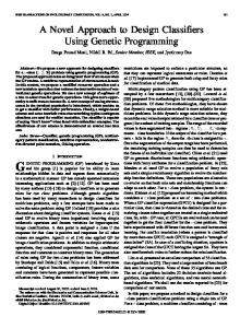
tree is close to the specified size, and only then terminals are chosen. Moreover, the predefined maximum size of the trees must not be violated. Each individual can be selected proportionally to its fitness value for the genetic operations: crossover and mutation. In this study, the selection method implements lexicographic parsimony pressure [30]. Like the tournament scheme, a random number of individuals are chosen from the population and the best of them is selected. The main difference is that if two individuals are equally fitted (according to Occam’s razor), the shortest one (the tree with less nodes) is chosen as the best one. Tree crossover and tree mutation are the genetic operators implemented as follows. In the tree crossover, random nodes are chosen from both parent trees, and the respective branches are swapped, creating two offspring. There is no bias towards choosing internal or terminal nodes as the crossing sites. In the tree mutation, a random node is chosen from the parent tree and substituted by a new random tree created with the terminals and functions available. This new random tree is created with the grow initialization method [28] and obeys the size restrictions imposed on the trees created for the initial generation. GP is terminated when the number of epochs exceeds a predefined threshold or one of the solutions fitness value meets the expected result. The brief procedure for genetic programming is outlined in Fig. 1.

1. Initialize the population by Full method. 2. For each individual repeat the following steps • Train the classifier with training samples, then, classify the test samples using feature groups in each individual. • Associate score to each individual. 3. Select the best individuals to generate new offspring. 4. Recombine and mutate the selected individuals. 5. Go to 2.

Fig. 1 Procedure for genetic programming.

5.

Classifiers

It is expected that the features selected by the scheme outlined above have a good performance on various types of classifiers. To test this, three powerful classifiers such as Linear Discriminant Analysis (LDA), Multi-LDA (MLDA), and Adaboost are considered. Although Fisher LDA was proposed in 1936 [31], its boundary is constructed based on a very powerful and efficient criterion (Fisher criterion). The LDA acts very robust and stable in some applications such as face recognition and 9

Neural Network World 1/12, 3-20

brain computer interface (BCI) [33], [36]. The multi-linear Discriminant Analysis (MLDA) is an efficient classifier which employs tensor properties to simplify the computation with acceptable accuracy [34]. The Adaboost [32] is a hybrid structure which uses several classifiers of different type to improve the accuracy. Both classifiers are easy to implement and are moderate in computational demand. In addition, it is straight forward to evaluate classification accuracy in both cases.

5.1

Fisher Linear Discriminant Analysis

The goal of LDA is to find a direction in the feature space in which the distance of the means relative to the within-class scatter, described by the within-class scatter matrix SW , reaches a maximum, thereby maximizing the class separability. This goal can be achieved by maximizing the following criterion with SB , the between scatter matrix: J(W ) =

W T SB W . W T SW W

(9)

The direction w that maximizes this criterion is determined as [33]: −1 W = SW (m1 − m2 ),

(10)

where m1 and m2 are the sample means for the two classes. This direction is optimal when the distribution of both classes is Gaussian and has the same scattering directions [33]. When the overlap between two classes increases, the LDA behaves very stable, because the boundary is formed based on all samples, not just marginal samples. The performance of some classifiers such neural networks, SVM and fuzzy classifier are so sensitive to marginal samples while the LDA is learned regarding between and within covariance matrices which involve all samples.

5.2

MLDA

The Multi-linear Discriminant Analysis (MLDA) was first proposed for the face recognition problem [34]. The distinctive property of this classifier is to preserve the data structure by catching inputs encoded as tensors. In traditional methods of face recognition, first, each image was vectorized, which projected to a very high dimensional space. Since the number of images in the database is far less than the number of feature dimension, the small sample size (SSS) problem [31] appeared, which lead to under-estimation parameters of a classifier. For example, in the face recognition using MLDA, each face (gray scale) is represented by two order tensors; therefore, the small sample size problem or the curse of dimensionality dilemma is neglected. In this study, the MLDA is employed because feature dimension is high (300) and this method can rapidly handle our data according to the tensor analysis. In the MLDA, objects are represented using a tensor and all computations are performed by tensor metrics. In addition, the transformation obtained in the MLDA is multi-linear, with a sub-transformation for each direction. If the k-order tensor is used to encode input data objects, the obtained transformation consists of k subtransformations. At each epoch of MLDA, the tensor objects are unfolded along 10

Sabeti M., Boostani R., Zoughi T.: Using genetic programming to select. . .

k-th direction (mode) and new objects are generated. The new objects are used to determine transformation in that direction. The key point is that, before unfolding objects in the mode k, all objects are transformed using the other k − 1 transformation. A special product called k-mode product is used to transform each object in the direction k. Since each transform depends on others, a mechanism named k-mode optimization is used to optimize the multi-linear transform. The between Sb and within Sw class scatter matrices in tensor representation are described as: Sb =

Nc ∑ Nc ∑ ¯c − X ¯ c )(X ¯c − X ¯ c )T (X i j i j

(11)

j=1 i=1

Sw =

Nc ∑ Nc i ∑ ¯ c )(Xi − X ¯ c )T , (Xi − X j j

(12)

j=1 i=1

where Nc and Nci are the number of classes and number of tensor objects in class ¯ c is the mean of i-th i, respectively. Xi is the i-th tensor object of class i and X j class.

5.3

Adaboost

The main idea of Adaboost is that a weak learning algorithm that performs just slightly better than random guessing can be boosted into an arbitrarily accurate and strong learning algorithm [32]. The Adaboost tries to boost a weak classifier in a serial manner. First, a uniform importance function is assigned to all training samples and the first weak learner is applied. Next, the weak learner tries to learn the misclassified samples which the previous learner could not classify. In other words, sensitivity of the next weak learner increases for the previous misclassified and decreases for the right classified samples in the previous iteration; therefore, each weak learner is forced to focus on the hard samples in the training set. Change of this sensitivity is performed based on the updating of the importance function called Dt (i), which is the importance of the sample i-th on the t-th iteration. Experimentally, the maximum number of weak learners (T ) can be adjusted by the user to avoid high computational complexity. In this study, the decision tree is chosen as a weak learner. One of the main ideas of the algorithm is to maintain a distribution or a set of weights over the training set. Each weak learner in the t-th iteration is defined as a hypothesis: ht : X → Y where X is the input vectors and Y are their labels. The error in the t-th iteration is defined as the number of misclassified samples, described as: εt = Pr [ht (xi ) ̸= yi ], i∼Dt

(13)

where ht is the t-th weak learner and εt numerates the number of samples that the t-th weak learner estimate their labels wrongly. Then, the Adaboost chooses a parameter αt ∈ R that intuitively measures the importance of ht that is determined as: ( ) 1 1 − εt αt = ln , (14) 2 εt 11

Neural Network World 1/12, 3-20

where αt is the weight assigned to ht . Finally, Dt is updated using the rule shown in Fig. 2. The final or combined classifier H is a weighted majority vote of the T -base classifiers.

1. Given: (x1 , y1 ), . . . , (xm , ym ) where xi ∈ X, yi ∈ Y = {−1, +1} 2. Initialize D1 (i) = 1/m. 3. For t = 1, . . . , T : • Train base learner using distribution Dt . • Get base classifier ht : X → R. • Choose αt ∈ R. t yi ht (xi )) • Update: Dt+1 (i) = Dt (i) exp(−α where Zt is a norZt malization factor (chosen so that Dt+1 will be a distribution).

4. Output the final classifier: (T ) ∑ H(x) = sign αt ht (x) t=1

Fig. 2 Procedure for Adaboost classifier.

6.

Computational Procedure

At first, EEG signals (20 channels) of fifteen schizophrenic patients and nineteen age-matched controls were recorded. The recorded signal of each channel was divided into short windows to preserve stationary property of each segmented signal. The window length was considered one second (to be stationary) and successive windows have a 50% overlap. Several features including the AR model coefficients (order 8), band power and fractal dimension were extracted from each frame. The extracted features from the successive windowed signals were arranged in successive feature vectors; there will be 15 features for each channel (8 features for AR coefficients, 4 for band power and 3 for fractal dimension); consequently, 300 features for each frame from all 20 electrodes are collected in each feature vector. In this phase, GP is employed for feature reduction so that each individual (or each tree) contains the group of features. In the feature selection phase, the features of each tree are used by Adaboost, MLDA, and LDA classifiers separately to learn the training samples, and the classification error on the test samples is returned as the fitness value. Once again the reduced features were fed into the classifiers, so that in all experiments, leave-one (subject)-out is used to estimate the classification error and prevent overfitting. It means that all extracted features of one subject were 12

Sabeti M., Boostani R., Zoughi T.: Using genetic programming to select. . .

considered as a test and the rest (extracted features of the remained cases) were employed to train the classifier. In this way, we do not have any correlation between the train and test sets to guarantee the generalization of the results. Moreover, leave-one-out is used because the number of cases were limited, otherwise k-times, k-folds cross validation would be a more proper method.

7.

Results and Discussions

In the first experiment, all the extracted features (300 features for each windowed signal) were applied to LDA, MLDA and Adaboost classifiers. One participant was considered as the test data and the other participants were considered as the train data. Each classifier is trained by the train data and the classification rate on the test data is determined. Tab. I shows the classification rate for each case separately through the leave-one (participant)-out process. As can be seen in Tab. I, the mean classification accuracy obtained by LDA, MLDA and Adaboost are 78%, 81%, and 82%, respectively. N1 LDA 94.53 MLDA 85.94 Adaboost 72.66 N10 LDA 98.82 MLDA 98.82 Adaboost 89.94 N19 LDA 57.40 MLDA 79.82 Adaboost 66.82 S9 LDA 78.20 MLDA 80.09 Adaboost 98.10

N2 96.89 88.89 92.44 N11 100 100 100 S1 47.37 47.37 68.42 S10 78.60 79.65 96.84

N3 85.47 88.27 45.81 N12 80.90 97.75 67.42 S2 66.08 58.59 86.78 S11 47.49 56.16 52.05

N4 60.50 59.66 69.75 N13 60.00 64.44 55.56 S3 87.84 87.84 94.14 S12 85.71 92.55 38.82

N5 98.51 98.51 100 N14 73.58 88.05 89.31 S4 91.67 90.48 92.26 S13 56.70 80.86 86.12

N6 98.65 97.97 88.51 N15 100 97.09 96.60 S5 51.27 65.19 34.18 S14 94.72 94.72 87.79

N7 61.96 96.74 100 N16 52.85 43.67 85.76 S6 42.86 30.77 79.67 S15 95.29 94.12 98.82

N8 N9 100 99.44 100 100 97.69 93.22 N17 N18 74.61 87.40 78.76 80.82 89.12 88.77 S7 S8 90.31 68.42 89.80 59.65 93.37 89.22 Mean ± Std 78.35 ± 18.69 80.97 ± 18.50 81.94 ± 18.37

Tab. I Results of LDA, MLDA and Adaboost classifiers on normal and schizophrenic subjects (N1 to N19 are normal subjects while S1 to S15 are schizophrenic patients). In the second experiment, genetic programming is used to reduce the complexity and remove the redundant features. The simulation parameters for genetic programming are brought in Tab. II. As it can be seen in Tab. II, the population with 50 trees was considered; the maximum allowed height of each tree is set to seven. In the initialization phase, features of a node are selected randomly, but the number of features of a node must not exceed five. Therefore, it is clear that each initial tree contains a different number of features. Typically, the GP procedure 13

Neural Network World 1/12, 3-20

is terminated after 100 epochs, but it is possible to stop the procedure when its accuracy is not changed significantly. The time complexity of GP depends on various factors such as size of population, number of epochs, time complexity of evaluation function, and number of training samples. If the accuracy of GP procedure is not changed significantly, the GP process is terminated before completion of maximum iteration threshold and hence it reduces the run time. The genetic programming parameters Population size 50 Initialization Full method Stopping criteria Maximum generation Selection Lexictour Crossover probability 0.8 Mutation probability 0.05 Maximum allowed height of a tree 7 Maximum allowed features of a node 5 Maximum allowed features of a tree 300 Tab. II The parameters used for genetic programming. As we can see from the results, GP reduced the classification error because it removed the redundant features. The algorithm is executed for 34 times that in each run, EEG signals of 33 participants are used to find the best subset of features. Finally, the best subset of features is used to classify unseen data. GP decreased the number of features approximately to half in each run. The selected features in each run are combined to find the final subset of features. The final number of features, after the intersection procedure, is 140 where it shows in each run, we obtain almost the same features. Investigating the final feature set it shows it contains all types of features (AR, band power and fractal dimension), with the most frequent AR coefficients and the least used fractal dimension. The selected features of each type are listed in Tab. III. Several operators can be used to obtain a composite feature set. These operators may be an intersection or union of the selected feature vectors, but maximum voting or feature weighting techniques also could be used. These operators were evaluated and finally we found out that the best choice is the intersection operator. Therefore, the final subset of features is considered as the intersection of the selected features in each run. Feature Type AR Band power Fractal dimension

# of selected features in the final feature set 84 35 21

Tab. III Selected number of features of each type by GP is shown separately. 14

Sabeti M., Boostani R., Zoughi T.: Using genetic programming to select. . .

Furthermore, decreasing the feature dimension enables the classifiers to learn more robust solutions and achieve better generalization performances. This is due to the fact that irrelevant feature components are eliminated by projection of the primary space to the optimal subspace. After feature reduction by GP, the classification rate is brilliantly improved to 82%, 84%, and 93% for the LDA, MLDA and Adaboost classifiers, respectively, as shown in Tab. IV. In order to illustrate the effectiveness of GP on the classification performance between two groups, the classification rate with and without applying GP along with their standard deviation are presented in Fig. 3. An interesting observation from the feature selection procedure is that most of the selected features belong to those channels which are located in the temporal and frontal lobes, covering most parts of limbic system in the brain. This result confirms the neuropsychological and neuroanatomical differences between controls and schizophrenic participants [1], and it also shows that the selected channels in the limbic area carry more discriminative information. Fig. 4 shows the final selected channels according to GP include Cz, C3 , T3 , T4 , Fp2 , F8 , T6 , O1 , O2 . Significant changes in the limbic system of control subjects with schizophrenic patients are observed in PET and fMRI images [35]. Hornero et al. [6] reported a similar work, analyzing a time series generated by twenty schizophrenic patients and twenty sex- and age-matched control subjects. They reported accuracies from 70–85% (depending on the nonlinear method used) for separating training and test sets. A remarkable enhancement has been achieved in this study when compared to the results obtained by Hornero et al. [6]. Moreover, in comparison with the generated time series [6], our approach has some advantages, including; (1) our approach is based on analyzing the EEG signals which can represent the discriminative spatio-temporal information on the scalp between the two groups while their approach just reflects the differences between cognitive activity of the two groups. (2) Their algorithms [6] are highly parameter dependant and tuning these parameters and finding the optimum threshold is hard while no prior knowledge or predefined threshold are needed in our approach. (3) In this research, most of the computation time is consumed by the training phase which is carried out offline and the recall phase is much faster than the method in [6]. To show the performance of GP feature selection technique, a well-known feature selection technique named Sequential Forward Selection (SFS) [31], [33] is applied to the extracted features. The SFS is an efficient technique in several applications but it highly suffers from lack of backtracking while genetic programming, by evolving its chromosomes in each generation, feeds an efficient backtracking process through its population. In other words, GP benefits a better global search than the SFS. To compare the performance of GP and SFS, both methods have been applied to the original features and the results are assessed in Tab. V. As we can see from the Tab. V, the GP achievements are superior to the SFS results. Furthermore, a reliable statistical test (student T-test) was applied on the achieved results in order to empirically confirm the significance of the classification improvements after the feature selection. Tab. VI shows the p-value before and after the feature selection for the three classifiers. Our results show the pvalue is less than 0.05 for Adaboost classifier, which confirms the validation of our 15

Neural Network World 1/12, 3-20

LDA MLDA Adaboost LDA MLDA Adaboost LDA MLDA Adaboost LDA MLDA Adaboost

N1 93.75 90.63 90.63 N10 94.67 98.82 91.67 N19 71.75 85.20 76.58 S9 87.68 75.83 98.10

N2 98.67 95.56 91.96 N11 98.84 100 100 S1 68.42 61.58 88.89 S10 78.95 75.09 86.48

N3 73.18 88.83 80.90 N12 80.90 98.88 75.00 S2 90.31 64.76 98.23 S11 86.94 62.03 93.58

N4 50.42 54.62 77.97 N13 50.00 64.44 71.11 S3 85.59 89.64 94.59 S12 86.02 93.17 100

N5 95.52 98.51 100 N14 69.81 89.31 84.81 S4 92.86 91.07 100 S13 65.79 81.58 100

N6 90.54 97.30 95.95 N15 97.57 95.63 100 S5 68.35 65.08 91.14 S14 95.38 94.72 100

N7 77.17 97.83 100 N16 47.47 47.78 88.61 S6 70.33 70.25 95.60 S15 96.47 93.53 96.47

N8 N9 100 96.05 100 100 100 89.77 N17 N18 80.31 93.15 91.71 86.03 100 97.80 S7 S8 91.84 65.66 89.80 52.88 96.94 97.99 Mean ± Std 82.07 ± 14.95 83.59 ± 15.76 92.67 ± 8.25

Tab. IV Results of LDA, MLDA and Adaboost classifiers on normal and schizophrenic subjects (N1 to N19 are normal subjects while S1 to S15 are schizophrenic patients) after feature selection.

LDA MLDA Adaboost

Genetic programming 82.07 ± 14.95 83.59 ± 15.76 92.67 ± 8.25

SFS 81.14 ± 19.47 81.54 ± 19.87 82.28 ± 18.00

Tab. V Comparison of GP and SFS feature selection techniques.

computation. Nevertheless, applying the GP feature selection did not provide any valid improvement for MLDA and LDA classification results. The main reason of Adaboost superiority is its ability to construct a non-linear and flexible boundary while preserving generalization of the results. In contrast, the linear classifiers are able to classify only linearly separable instances. The higher accuracy of Adaboost addresses the hard margin between the extracted features of the two classes. The performance of Adaboost can be highly affected by noisy features; therefore, eliminating noisy features dramatically improved the performance of Adaboost; while LDA family classifiers are more robust to noisy features, hence, their effectiveness did not change significantly after the feature selection. It should be noted that for each psychiatric disease, there are some different drugs which affect EEG signals. It was impossible to stop patients’ medicine for our research; therefore, we asked the psychiatrist to use those drugs (dopamine blocker group) which have minimum affect on EEG signals. Mostly, preprocessing of data such as normalization could affect performance of the classifiers. This was investigated for this particular data set and no significant changes were observed. 16

Sabeti M., Boostani R., Zoughi T.: Using genetic programming to select. . .

Fig. 3 Classification result along with standard deviation is shown for schizophrenic and control subjects by LDA, MLDA and Adaboost classifiers. Shaded bars show the results without feature reduction, white bars show the results using GP.

Fig. 4 Visualization of the selected channels by GP on the scalp. Dark gray shows the selected channels. At the end, applying GP on the features increased the performance of all classifiers and the Adaboost was introduced as the most effective classifier compared to the LDA and MLDA for distinguishing schizophrenic and control subjects. In order to improve this performance, we can employ the two-layer weighted-LDA weightednearest neighbor classifier [38] or adaptive distance immune system-based classifier [39] which prove their efficiency empirically on the standard datasets. In some 17

Neural Network World 1/12, 3-20

Classifier LDA MLDA Adaboost

p-value p > 0.05 p > 0.05 p < 0.05

Tab. VI The statistical test result. researches EEG signals were recorded in presence of auditory stimulus, and after extracting the evoke related potential from the background EEG, proper features such as latency and amplitude were used to distinguish the schizophrenic subjects from the controls [40], but here we analyze the natural EEG (without any stimulus) to see whether any significant indicator is observed between the two groups to classify them or not.

8.

Conclusions

This study shows that EEG signals can be an efficient tool for distinguishing schizophrenic and control participants. EEG signals are preprocessed, then the descriptive features represent the captured information inside the signals in different domains to highlight their differences. Three well-known classifiers, LDA, MLDA and Adaboost, were trained using leave-one (patient)-out procedure for training in order to remove correlation between the train and test sets. Satisfactory results are fairly obtained by distinguishing the patterns. For further improvement, genetic programming is used for removing redundant and noisy features; the results achieved by Adaboost classifier are considerably enhanced due to Adaboost capability to fit a non-linear boundary among the filtered features while preserving generalization between the train and test results. Experimental results illustrate the effectiveness of the proposed approach that can be a complementary tool to help psychiatrists for more accurate diagnosing schizophrenic patients.

References [1] American Psychiatric Association: diagnostic and statistical manual of mental disorders: DSM-IV, Washington DC, 1994. [2] Niedermeyer E., Silva F. L. D.: Electroencephalography basic principles, clinical application and related fields (fourth edition), Lippincott Williams & Wilkins, 1999. [3] Roschke J., Fell J., Beckmann P.: Nonlinear analysis of sleep EEG data in schizophrenia: Calculation of the principal Lyapunov exponent, Psychiatry Res., 56, 1995, pp. 257-268. [4] Koukkou M., Lehmann D., Wackermann J.: Dimensional complexity of EEG brain mechanisms in untreated schizophrenia, Biol. Psychiatry, 33, 1993, pp. 397-407. [5] Jeong J., Kim D. J., Chae J. H., Kim S. Y., Ko H. J., Paik I. H.: Nonlinear analysis of the EEG of schizophrenics with optimal embedding dimension, Med. Eng. Phys., 20, 1998, pp. 669-676. [6] Hornero R., Ab´ asolo D., Jimeno N., S´ anchez C. I., Poza J., Aboy M.: Variability, regularity and complexity of time series generated by schizophrenic patients and control subjects, IEEE Transaction on Biomedical Engineering, 53, 2, 2006, pp. 210-218.

18

Sabeti M., Boostani R., Zoughi T.: Using genetic programming to select. . .

[7] Sabeti M., Boostani R., Katebi S. D., Price G. W.: Selection of Relevant Features for EEG Signal Classification of Schizophrenic Patients, Biomedical Signal Processing and Control, 2, 2007, pp. 122-134. [8] Boostani R., Sadatnezhad K., Sabeti M.: An Efficient Classifier to Diagnose of Schizophrenia Based on the EEG Signals, Expert Systems With Applications, July 2008. [9] Rosenberg S., Weber N., Crocq M. A., Duval F., Macher J. P.: Random number generation by normal, alcoholic and schizophrenic subjects, Psychol Med., 20, 1990, pp. 953–960. [10] Pressman A., Peled A., Geva A. B.: Synchronization analysis of multi-channel EEG of schizophrenic during working-memory tasks, IEEE proceedings of the 21st convention of the electronics engineering, Israel, 2000, pp. 337-341. [11] International Statistical Classification of Diseases and Health Related Problems (The) ICD10 Second Edition, World Health Organization, 2005. [12] Semlitch H. V., Anderer P., Schuster P., Presslich O.: A solution for reliable and valid reduction of ocular artifacts applied to the P300 ERP, Psychophysiology A, 23, 1986, pp. 696-703. [13] Schwilden H.: Concepts of EEG processing: from power spectrum to bispectrum, fractals, entropies and all that, Best Practice & Research Clinical Anaesthesiology, 20, 1, 2006, pp. 31-48. [14] Shen Y., Olbrich E., Achermann P., Meier P. F.: Dimensional complexity and spectral properties of the human sleep EEG, Clinical Neurophysiology, 114, 2003, pp. 199-209. [15] Pfurtscheller G., Neuper C.: Motor imagery and direct brain-computer communication, In proceedings of the IEEE, 89, 7, 2001, pp. 1123 -1134. [16] Obermaier B., Neuper C., Guger C., Pfurtscheller G.: Information transfer rate in a fiveclasses brain-computer interface, IEEE Transactions on Rehabilitation Engineering, 9, 3, 2001, pp. 283-288. [17] Esteller R., Vachtsevanos G., Echauz J., Litt B.: A comparison of waveform fractal dimension algorithms, IEEE Transaction on Circuits and Systems I: fundamental theory and applications, 48, 2, 2001, pp. 177-183. [18] Liu J. Z., Yang Q., Yao B., Brown R. W., Yue G. H.: Linear correlation between fractal dimension of EEG signal and handgrip force, Biological Cybernetics, 93, 2, 2005, pp. 131-140. [19] Galka A.: Topics in nonlinear time series analysis with implication for EEG analysis, World Scientific, 2000. [20] Stoica P., Moses R. L.: Introduction to spectral analysis, Prentice Hall, 1997. [21] Broersen P. M. T., Wensink H. E.: On finite sample theory for autoregressive model order selection, IEEE Transaction on Signal Processing, 41, 1993, pp. 194-204. [22] Niedermeyer E., da Silva F. L.: Electroencephalography, Basic Problems, Clinical Applications, and Related Fields, Lippincott Williams & Wilkins, Philadelphia, Pa, USA, 4th edition, 1999. [23] Higuchi T.: Approach to an irregular time series on the basis of the fractal theory, Physica D, 31, 1988, pp. 277-283. [24] Katz M.: Fractals and the analysis of waveforms, Comput Biol Med, 18, 3, 1988, pp. 145-156. [25] Petrosian A.: Kolmogorov Complexity of Finite Sequences and Recognition of Different Preictal EEG Patterns, In proceeding of the IEEE Symposium on Computer-Based Medical Systems, 1995, pp. 212-217. [26] Muni D. P., Pal N. R., Das J.: Genetic programming for simultaneous feature selection and classifier design, IEEE Transaction on Systems, Man and Cybernetics – Part B: Cybernetics, 36, 1, 2006, pp. 106-117. [27] Blum A. L., Langley P.: Selection of relevant features and examples in machine learning, Artificial Intelligence, 97, 1997, 245-271. [28] Langdon W. B., Poli R.: Foundations of genetic programming, Springer-Verlag, 2002.

19

Neural Network World 1/12, 3-20

[29] Yu T., Riolo R., Worzel R.: Genetic programming theory and practice III, Springer-Verlag, 2006. [30] Luke S., Panait L.: Lexicographic parsimony pressure, In: Langdon W. B., Cant´ u-Paz E., Mathias K., Roy R., Davis D., Poli R., Balakrishnan K., Honavar V., Rudolph G., Wegener J., Bull L., Potter M. A., Schultz A. C., Miller J. F., Burke E., Jonoska N., editors, Proceedings of GECCO-2002, San Francisco, CA. Morgan Kaufmann, 2002, pp. 829-836. [31] Webb A. R.: Statistical pattern recognition (second edition), John Wiley and Sons Ltd., 2002. [32] Schapire R. E.: The boosting approach to machine learning an overview, In: Denison D. D., Hansen M. H., Holmes C., Mallick B., Yu B., editors, Nonlinear Estimation and Classification, Springer, 2003. [33] Duda R. O., Hart P. E., Stork D. G.: Pattern classification (second edition), Wiley Interscience, 2001. [34] Yan S., Xu D., Yang Q., Zhang L., Tang X., Zhang H-J.: Multilinear Discriminant Analysis for Face Recognition, IEEE Trans. on Image Processing, 16, 1, Jan. 2007, pp. 212–220. [35] Sadock B. J., Sadock V. A.: Kaplan & Sadock’s Comprehensive Textbook of Psychiatry, Lippinkott Williams & Walkins, 8th edition, 2005. [36] Boostani R., Graimann B., Moradi M., Pfurtscheller G.: A comparison Approach Toward Finding the Best Features and Classifiers in Cue-based BCI, Springer journal of Medical & Biological Engineering & Computing, 45, 4, Feb. 2007, pp. 403-412. [37] Sabeti M., Katebi S. D., Boostani R.: Entropy and Complexity Measures for EEG Signal Classification of Schizophrenic and Control Participants, Artificial Intelligence in Medicine, 47, 2009, pp. 263-274. [38] Boostani R., Dehzangi O., Jarchi D., Zolghadri Jahromi M.: An efficient pattern classification approach: combination of weighted LDA and weighted nearest neighbor, Journal of Neural Network World, 20, 5, 2010, pp. 621-635. [39] Zare A., Zolghadri Jahromi M., Boostani R.: An Adaptive Distance Immune System Classifier, Neural Network World, (In Press) 2010. 20, 5, 2010, pp. 637-650. [40] Callaway E., Jones R. T., Donchin E.: Auditory evoked potential variability in schizophrenia, Electroencephalography and Clinical Neurophysiology, 29, 5, November 1970, pp. 421-428.

20