Variance Reduction in Simulation of Multiclass Queueing ... - CiteSeerX

Variance Reduction in Simulation of Multiclass Queueing Networks Shane G. Henderson∗ School of Operations Research and Industrial Engineering, Cornell University Ithaca, NY 14850 Sean P. Meyn† Department of Electrical and Computer Engineering University of Illinois-Urbana/Champaign Urbana, IL 61801, U.S.A. March 26, 2003

Abstract We use simulation to estimate the steady-state performance of a stable multiclass queueing network. Standard estimators have been seen to perform poorly when the network is heavily loaded. We introduce two new simulation estimators. The first provides substantial variance reductions in moderately-loaded networks at very little additional computational cost. The second estimator provides substantial variance reductions in heavy traffic, again for a small additional computational cost. Both methods employ the variance reduction method of control variates, and differ in terms of how the control variates are constructed. ∗ †

Work supported in part by NSF grant DMI-0224884 Work supported in part by NSF grants DMI-0224884 and ECS 940372

1

1

Introduction

A multiclass queueing network is a network of service stations through which multiple classes of customers move. Each customer class can have different service-time characteristics at a single service station. Multiclass queueing networks are of great interest in a large variety of applications [Bertsekas and Gallagher, 1987, Lavenberg, 1983, Buzacott and Shanthikumar, 1993, Gershwin, 1993] because of their tremendous modeling flexibility. Perhaps the most common reason for modeling a system using a multiclass queueing network is to try to determine a suitable operating policy for the network. An operating policy is a policy that determines which customers should be worked on at which times. For example, if there are multiple customer classes at a single service station, then which class should the station work on? In order to make comparisons between operating policies, one must define a suitable performance measure, such as expected steady-state work in process, or expected steadystate throughput etc. For certain broad classes of networks one can compute certain performance measures analytically [Jackson, 1963, Baskett et al., 1975, Kelly, 1979, Harrison and Williams, 1990, 1987], or one can turn to numerical computation [Schweitzer, 1984, Neuts, 1994, Dai and Harrison, 1992, Shen et al., 2002]. In general, however, these approaches are either infeasible, or intractable due to the high complexity of network models. Some results are available in the form of bounds on performance measures through the construction of linear programs [Kumar and Kumar, 1994, Bertsimas et al., 1994, Kumar and Meyn, 1996, Schwerer, 2001, Morrison and Kumar, 1999]. Unfortunately, these bounds are often quite loose, and so it can be difficult to compare operating policies based on such bounds alone. It is natural then, to turn to simulation. Given that one is going to simulate many different operating policies, it is important that any simulation return relatively accurate answers as quickly as possible. This suggests the need for variance-reduction techniques that can increase the accuracy in simulation results for a given computational budget. Another reason for desiring efficient simulation techniques is that that the network under consideration is often moderately to heavily loaded, in the sense that some of the resources of the network are close to full utilization.

2

It has been noted that, in such settings, simulation can take a tremendously long time to return accurate estimates of performance [Whitt, 1989, Asmussen, 1992]. So we are strongly motivated to seek special variance-reduction techniques for multiclass networks. In this paper we develop two such variance-reduction techniques. Both are based on the approximating martingale process method [Henderson and Glynn, 2002, Henderson, 1997], which is a specialization of the method of control variates; see, for example, Law and Kelton [2000] for an introduction to control variates. This paper is an outgrowth of Henderson and Meyn [1997]. The methods introduced there and here have since seen further development in Henderson et al. [2003] and Borkar and Meyn [2003]. Although our presentation concentrates on the estimation of the mean steady-state number of customers (of all classes) in the system, our methods may be tailored to the steady-state estimation of any linear function of the individual customer-class populations. In particular, we can also estimate, for instance, the mean steady-state number of customers of a particular class present in the system. In Section 2 we describe our model of a multiclass-queueing system. We also review Poisson’s equation and explain its importance in our context. In particular, we wish to approximate the solution to Poisson’s equation to construct efficient simulators. In Section 3, we explore quadratic forms as approximations to the solution to Poisson’s equation. Computational results are given for the resulting simulation estimator, which we term the quadratic estimator. The quadratic estimator significantly outperforms a more standard simulation estimator in lightly to moderately-loaded networks. In heavily-loaded networks, the difference between the performance of the two estimators closes, although the quadratic estimator still provides variance reductions that would significantly reduce the computational effort involved in exploring a class of operating policies. In Section 4, we explore alternative approximations to the solution to Poisson’s equation based on the concept of a fluid limit. The resulting simulation estimator, the fluid estimator, yields significant variance reductions in heavily-loaded networks, and modest variance reductions in less heavily-loaded networks. For a given simulation run-length, it is slightly more expensive to compute than the standard estimator, so that the issue of variance reduction versus computational effort needs to be considered [Glynn and Whitt,

3

1992]. We discuss the choice of simulation estimator for a given network in Section 5.

2

Multiclass Queueing Networks

Consider a system consisting of d stations (or machines) and ` classes of customers (or jobs). Class i customers require service at station s(i). Upon completion of service at station s(i), a class i customer becomes a class j customer with probability R ij , and exits the system with probability 4

Ri0 = 1 −

` X

Rij .

j=1

The service times for class i customers are assumed to form an i.i.d. sequence of exponentially distributed r.v.’s with mean µ−1 i . Class i customers arrive exogenously to station s(i) according to a Poisson process with rate λi (which may be zero). The Poissonarrival processes and the service-time processes are mutually independent. We let µ denote the `-dimensional vector of service rates, and λ the d-dimensional vector of arrival rates. Unless otherwise stated, all vectors are assumed to be column vectors. We require that the routing matrix R = (Rij : 1 ≤ i, j ≤ `) be transient, so that the following inverse exists: (I − R)−1 =

∞ X

Rk .

k=0

This ensures that all customers that enter the system will eventually leave, and we can also be assured that there is a unique solution γ ≥ 0 to the traffic equations, 0 = λ − γ + R0 γ,

(1)

where R0 denotes the transpose of the matrix R. We assume throughout that γi > 0 for all i. Figure 1 illustrates an example with d = 2 stations, ` = 3 customer classes, and a single exogenous arrival process (two of the arrival rates are zero). Customer classes 1 and 3 are served at Station 1, so that s(1) = s(3) = 1. Similarly s(2) = 2. The routing values Rij are zero except for R12 = R23 = 1. Let Xi (t) denote the number of class i customers present in the system at time t, and let X(t) = (Xi (t) : 1 ≤ i ≤ `) be the vector of customer populations at time t. Let Vi (t) 4

α1 µ1

µ2



  



   µ3

Figure 1: A multiclass network with d = 2 stations and ` = 3 customer classes. denote the fraction of station s(i)’s effort allocated to serving customers of class i at time t, and let V (t) denote the corresponding vector quantity. We must have Vi (t) ≥ 0 for all P i and t, and i:s(i)=s Vi (t) ≤ 1 for all s and t, i.e., a station s can never allocate negative

effort, or more than unit effort, to the classes {i : s(i) = s} that are served at the station.

For the network in Figure 1 for example, suppose that at time t Machine 1 is serving Class-3 jobs, and Machine 2 is empty. Then V (t) = (0, 0, 1)0 . We require the operating policy adopted by stations to be stationary, non-idling, and 0 − 1. We next define and explain each of these terms. By stationary, we mean that V (t) is a deterministic function of X(t), so that the workload allocations depend only on the current customer-class levels. This allows the modeling of preemptive priority policies, for example, but precludes the modeling of policies such as FIFO which rely on additional information such as the order in which customers arrive to a station. By non-idling, we mean that if

P

i:s(i)=s Xi (t)

> 0, then

P

i:s(i)=s Vi (t)

= 1, i.e., if

there are customers present at station s at time t, then the station allocates all of its effort at that time. By 0 − 1, we mean that at any given station, at most one class receives service at any given time. This assumption is applied only for notational convenience. The estimators we derive may also be applied to networks controlled by randomized or processor-sharing policies. With the above structure in place, we may conclude that X = (X(t) : t ≥ 0) is a

5

time-homogeneous continuous-time Markov chain. However, we prefer to work in discrete time because it simplifies the analysis. So we first rescale time so that e0 (λ + µ) = 1, where e denotes a vector of ones. Then we uniformize; see, e.g., Ross [1996, p. 282]. Uniformization is a process that allows us to study the continuous-time process X through a related discrete-time process Y = (Y (n) : n ≥ 0). Define τ0 = 0 and let the times {τn : n ≥ 1} correspond to epochs when either arrivals, real service completions, or virtual service completions occur in the uniformized process. For n ≥ 0, let Y (n) = X(τ n ) and W (n) = V (τn ). Then the process Y = (Y (n) : n ≥ 0) is a discrete-time Markov chain evolving on a (countable) state space S that is a subset of {0, 1, 2, ...}` . Example 1:

For the M/M/1 queue, Y is a Markov chain on {0, 1, 2, . . .} with transition

matrix P , where

Pij = (µ + λ)−1

   λ if j = i + 1,  

µ if j = max(i − 1, 0), and     0 otherwise.

Our goal is to estimate α, the steady-state mean number of customers in the system, 4

i.e., the steady-state mean of |Y (0)| = e0 Y (0) (i.e. | · | is the L1 norm). To ensure (among other things) that α exists and is finite, we make a certain assumption (A) below. The assumption (A) is known as a Lyapunov, or Foster-Lyapunov, condition. Intuitively, the function V represents energy, and (3) indicates that there is an expected loss in energy for states y that are “large.” This then ensures that energy never gets too large, and so the chain remains stable. For any function V on IR`+ we define 4

P V (y) = Ey V (Y (1)),

∆V (y) = P V (y) − V (y),

y ∈ S,

4

where Ey (·) = E(· | Y (0) = y). Intuitively, P V (y) (∆V (y)) represents the expected energy (expected change in energy) one step from now, assuming that the chain is currently in state y. (A) There exists a function V : IR`+ → IR+ satisfying 6

1. V is equivalent to a quintic in the sense that for some δ < 1, δ(|y|5 + 1) ≤ V (y) ≤ δ −1 (|y|5 + 1); and

(2)

2. for some η > 0, and all y, ∆V (y) = P V (y) − V (y) ≤ −|y|4 + η.

(3)

Continuation of Example 1: For the M/M/1 queue, we may take V (y) = b 0 y 5 , with b0 a 4

sufficiently large constant, and then (A) is satisfied as long as ρ = λ/µ < 1. In general, this condition will be satisfied if the stability-linear program of Kumar and Meyn [1996] admits a solution, generating a co-positive ` × ` matrix Q. In this case, the function V may be taken as V (y) = (y 0 Qy)5/2 . Alternatively, if a fluid model is stable, and we define κ = inf{n ≥ 1 : Y (n) = 0}, then the function V (y) = Ey

κ X

|Y (k)|4

k=0

is bounded as in Condition 1 [Dai and Meyn, 1995], and this function is known to satisfy Condition 2 [Meyn and Tweedie, 1993, p. 338]. Under the assumption (A), the chain Y possesses a unique stationary distribution π, and Eπ |Y (0)|4 ≤ η < ∞ [Meyn and Tweedie, 1993, p. 330], where 4

Eπ ( · ) =

Z

E( · |Y (0) = y)π(dy). S

Hence, in particular, the steady-state mean number of customers α = Eπ |Y (0)| < ∞. The Lyapunov condition (A) is stronger than is strictly necessary to ensure that α = Eπ |Y (0)| is finite. A “tighter” requirement is that there is a function h : IR`+ → IR+ satisfying ∆h (y) = P h(y) − h(y) ≤ −|y| + η

(4)

for all y ∈ S and some constant η > 0. Given such a function, Theorem 14.3.7 of Meyn and Tweedie [1993] allows us to conclude that α = Eπ |Y (0)| ≤ η.

7

One might then ask whether the inequality in (4) can be made an equality, thereby yielding a tighter upper bound η on α. In such a case we would have ∆h∗ (y) = P h∗ (y) − h∗ (y) = −|y| + η.

(5)

This equation is known as Poisson’s equation. If h∗ is a solution to Poisson’s equation, then it is easy to see that h∗ + c is also a solution for any constant c. In fact, Proposition 17.4.1 of Meyn and Tweedie [1993] shows that any two π-integrable solutions to Poisson’s equation must differ by an additive constant, in the sense that for all y in a set A with π(A) = 1, h1 (y) − π(h1 ) = h2 (y) − π(h2 ) where, for a real-valued function g : S → IR, we denote π(g) =

R

S g(y)π(dy). P One may estimate α using α(n) = |Y¯ (n)|, where Y¯ (n) = n−1 n−1 i=0 Y (i), the mean num4

4

ber of customers in the system up to time n. The following result is a special case of Theorem 17.0.1 of Meyn and Tweedie [1993], and shows that the estimator α(n) is consistent, and satisfies a central limit theorem.

Theorem 1 Suppose that (A) holds. Then α(n) → α almost surely (a.s.), and furthermore, n1/2 (α(n) − α) ⇒ σN (0, 1), as n → ∞. The time-average variance constant (TAVC) σ 2 is given by σ 2 = E[h(Y )(|Y | − E|Y |)] − Var |Y |, where Y is distributed according to the stationary distribution π, and h solves Poisson’s equation; see (5). As noted in the introduction, it has been observed that simulation can take a very long time to yield accurate answers for heavily-loaded networks [Asmussen, 1992, Whitt, 1989]. This problem is exhibited in our framework through the TAVC. Our simulation experiments indicate that the TAVC grows rapidly as the network becomes heavily loaded. Our next result lends further weight to these observations. Consider a multiclass queueing system consisting of a single station and (possibly) multiple customer classes. Suppose that the service rates µ and arrival rates λ are such 8

that e0 M −1 (I − R0 )−1 λ = 1, where M = diag(µ). (This corresponds to a situation where the resources of the network are exactly matched by the demand.) Now consider a family of queueing systems indexed by ρ ∈ (0, 1), where the ρth system has arrival rate vector λ(ρ) = ρλ. For the sake of clarity, we occasionally suppress dependence on ρ. For a given vector of buffer levels y, let f (y) = d0 y be a measure of the work in the system, where d0 = e0 M −1 (I − R0 )−1 = e0 Q, and Q = M −1 (I − R0 )−1 . Intuitively, f (y) measures that total expected amount of processing required to completely serve all of the customers presently in the system as given by y. Let σf2 (ρ) be the TAVC associated with the estimator f (Y¯ (n)) = d0 Y¯ (n), and let σi2 (ρ) be the TAVC associated with Y¯i (n) (i = 1, . . . , `). If Σρ denotes the time-average covariance matrix of Y , then σf2 (ρ) = d0 Σρ d and σi2 (ρ) = e0i Σρ ei , where ei denotes the ith basis vector. The proof of the following result may be found in the appendix. Theorem 2 Consider the family of multiclass queueing systems above under any nonidling work-allocation policy. Then the following are true for each ρ < 1. 1. Assumption (A) holds with the function bρ f 5 for some sufficiently large constant bρ , and the TAVCs σf2 (ρ) and σi2 (ρ) (i = 1, . . . , `) are finite. 2. The solution to Poisson’s equation for the estimator f (Y¯ (n)) is given by h(y; ρ) =

f 2 (y) + c0ρ y, 2(1 − ρ)

where the vector cρ is of the order (1 − ρ)−1 . Furthermore, there exist constants A, B > 0 (independent of ρ) such that for ρ sufficiently close to 1, A B ≤ σf2 (ρ) ≤ , 4 (1 − ρ) (1 − ρ)4

9

and finally trace Σρ =

` X

σi2 (ρ) ≥

i=1

for some constant

A0

A0 (1 − ρ)4

(again, independent of ρ).

Theorem 2 shows that trace Σρ is of the order (1 − ρ)−4 as ρ → 1, and this suggests, although it does not necessarily prove, that the TAVC e0 Σρ e of the standard estimator α(n) is of the same order. We have already mentioned that our simulation experiments also indicate that α(n) has high variance in heavily-congested networks. Therefore, there is strong motivation for identifying alternative estimators to α(n) that can improve performance in heavy traffic. The key to these estimators is Poisson’s equation. If h∗ is π-integrable, then by taking expectations with respect to π in (5), we see that α = η. Therefore, if the solution to Poisson’s equation is known, then so is α. In general then, we cannot expect to know the solution to Poisson’s equation. But what if an approximation is known? If the approximation h is π-integrable, then π(∆h ) = 0, i.e., ∆h (Yn ) has steady-state mean 0, and so one might consider using ∆h in building a simulation control variate in estimating α. In particular, one might consider using the controlled estimator n−1

αc (n) = α(n) +

βX ∆h (Y (i)), n

(6)

i=0

where β is an adjustable constant. If h = h∗ and we take β = 1, then αc (n) = α, and we obtain a zero-variance estimator of α. In general, we can expect useful variance reductions using the estimator α c (n) provided that h is a suitable approximation to the solution to Poisson’s equation. We will discuss the choice of the constant β later. For more details on this approach to variance reduction see Henderson and Glynn [2002], Henderson [1997], Henderson et al. [2003], Borkar and Meyn [2003]. So how should one go about determining an approximation to the solution h ∗ to Poisson’s equation? It is known that for any ‘reasonable’ policy, the function h∗ is equivalent to a quadratic, in the sense of (2) (see Kumar and Meyn [1996], Meyn [1997, 2001] and The-

10

orem 3 below). So it is reasonable to search for a quadratic function h that approximately solves (5).

3

A Quadratic Approximation

We begin this section by demonstrating the general ideas of the approach on the stable M/M/1 queue. Continuation of Example 1: Recall that the solution to Poisson’s equation is equivalent to a quadratic. So it is reasonable to approximate the solution h∗ to Poisson’s equation by a quadratic function. In the linear case h(y) = y, we have that ∆h (y) = λ − µw, where w = I(y > 0) (I(·) is the indicator function that is 1 if its argument is true and 0 otherwise) represents the only non-idling policy: The server works when customers are present, and idles when customers are not present. Taking expectations with respect to π, we see that the expected fraction of time that the server is working is Eπ W (0) = λ/µ, and this is the result expected by work conservation. Taking the pure quadratic h(y) = ay 2 , we have ∆h (y) = 2ay(λ − µ) + aλ + aµw.

(7)

We now choose a = (µ − λ)−1 /2 to ensure that the coefficient of y is −1. We could then use the right-hand side of (7) as a control variate as in (6). However, it is instructive (and useful) to adopt a slightly different approach where we avoid estimation of the variable w, and replace it by its known steady state mean Eπ W (0) = π(w) = λ/µ. We may then use the controlled estimator Y¯ (n) + β(−Y¯ (n) + 2λa). This estimator is in fact equal to the estimator Y¯ (n) + β∆h∗ (Y¯ (n)), with h∗ (y) = a(y 2 + y), the solution to Poisson’s equation. Hence if β = 1, this estimator has zero variance. We turn now to the general case. We assume throughout this section that the assumption (A) is in place, so that the network is stable, and all steady-state expectations that

11

we use exist. A similar development for reentrant lines may be found in Henderson and Meyn [1997]. Since the solution to Poisson’s equation is equivalent to a quadratic, it is reasonable to use h(y) = y 0 Qy + q 0 y, for some symmetric matrix Q and vector q. This approach was originally proposed in Kumar and Meyn [1996], based on the prior approaches to bounding network performance presented in Kumar and Kumar [1994], Bertsimas et al. [1994], Down and Meyn [1994]. We first consider the linear part of the function, and then turn to the quadratic terms. Consider the function hj (y) = yj for some j. Then, letting w denote the work allocation vector corresponding to the vector y, ∆hj (y) = λj − µj wj +

X

µi wi Rij .

(8)

i

Denote by x ¯ the vector (µi Eπ Wi (0) : 1 ≤ i ≤ `). Taking expectations with respect to π in (8) and writing the equations (one for each j) in vector form, we obtain 0=λ−x ¯ + R0 x ¯. Since the solution to (1) is unique, we conclude that Eπ Wj (0) = γj /µj . Thus by considering linear functions we have shown that the usual traffic conditions hold. Now consider the function hjk (y) = yj yk for j 6= k. Then, ∆hjk (y) = λj yk + λk yj − µj wj yk − µk wk yj X + µi wi (Rij yk + Rik yj ) − µj wj Rjk − µk wk Rkj .

(9)

i

Notice that (9) is a nonlinear expression in y, due to the presence of the w terms. We would prefer to work with linear expressions. To this end, introduce the variables Zij (n) = Wi (n)Yj (n), and let z¯ij = Eπ Wi (0)Yj (0) for 1 ≤ i, j ≤ `. Under our assumptions on the policy it follows that Z(n) is a fixed, deterministic function of Y (n). Furthermore, let y¯j = Eπ Yj (0). Taking expectations with respect to π in (9), we obtain 0 = λj y¯k + λk y¯j − µj z¯jk − µk z¯kj +

X

µi (Rij z¯ik + Rik z¯ij ) − γj Rjk − γk Rkj .

i

12

(10)

Now, the non-idling condition implies that whenever yj > 0 so that work is present at station s(j), X

wi = 1,

i:s(i)=s(j)

so that station j allocates all of its effort. Hence, for any value of y j , including 0, yj =

X

w i yj ,

i:s(i)=s(j)

and consequently, y¯j =

X

z¯ij .

(11)

i:s(i)=s(j)

Therefore, if we let z¯ be a column vector containing the z¯jk ’s, then the expression (10) may be written as u0jk z¯ = cjk , for a suitably-defined column vector ujk and constant cjk . By considering the function hjj (y) = yj2 , we obtain 0 = 2γj + 2λj y¯j − 2µj z¯jj + 2

X

µi Rij z¯ij ,

i

for j = 1, . . . , `, and again these equations can be written as u0jj z¯ = cjj for suitably defined ujj and cjj . We obtain one equation for each 1 ≤ j ≤ k ≤ `, so that in all there are `(` + 1)/2 equations of the form u0jk z¯ = cjk . If we now write the vectors {ujk } as columns in a matrix U , and the values {cjk } in a vector c, these equations can be written as U 0 z¯ = c. The matrix U has `2 rows, and `(` + 1)/2 columns. Although we began with expressions involving the Markov chain Y , we are now working with the Markov chain Z = (Z(n) : n ≥ 0). Therefore, it is useful to express the function |y| as p0 z, for some vector p. In particular, pij = 1 if s(i) = s(j), and 0 otherwise. In view Pn−1 ¯ ¯ Z(i). of (11), the estimator α(n) may be written as p0 Z(n), where Z(n) = n−1 i=0 So define the quadratic estimator as αq (n)

=

4

¯ ¯ p0 Z(n) + βν 0 (U 0 Z(n) − c)

=

¯ (p + βU ν)0 Z(n) − βν 0 c,

where ν is a vector of coefficients. This is again of the form αq (n) = |Y¯ (n)| + β∆h (Y¯ (n)), 13

(12)

where h is a quadratic, h(y) = y 0 Qy + ζ 0 y for some matrix Q and vector ζ. However in the case of networks, we can only hope that h approximately solves Poisson’s equation, in the sense that P h(y) − h(y) = −d(y) + αd , with d( · ) ≈ | · |. Let us assume (for now) that β = 1. The variance of (12) is then given by (p + U ν)0 Λn (p + U ν),

(13)

¯ where Λn is the covariance matrix of Z(n). But under appropriate initial conditions and ¯ assuming (A) holds, Λn ∼ Λ/n, where Λ is the time-average covariance matrix for Z(n). Then (13) is asymptotically given by 4

n−1 kp + U νk2Λ = n−1 (p + U ν)0 Λ(p + U ν).

(14)

Standard control variate methodology suggests that one could estimate the covariance matrix Λ (or U 0 ΛU ), and then choose ν to minimize the vector norm (14) [Law and Kelton, 2000, p. 609]. However, as cautioned in Law and Kelton [2000], there is the danger of a variance increase associated with the additional estimation of the covariance matrix. The “loss factor” is discussed in Lavenberg and Welch [1981] and Nelson [1990] for terminating simulations, and in Loh [1994] for steady-state simulation. The loss factor can become an issue when many control variables are used (as is potentially the case here). Rather than attempt to determine an optimal selection of control variables from those at our disposal, we instead choose to avoid the issue altogether by preselecting ν, and then using a standard approach to select the single parameter β. See Henderson and Meyn [1997] for further discussion related to this point. From (14), it is “optimal” to choose ν to minimize kU ν + pkΛ . Since Λ is unknown prior to the simulation, we instead choose ν to minimize kU ν + pki for some Li norm k · k. This problem can be solved using linear programming if i is chosen to be 1 or ∞, or using least-squares methods if i = 2. In addition, for some workload policies, for example preemptive priority policies, it is known that z¯ij = 0 for some i and j. In this case, we may modify the norm used in the minimization slightly to ignore the cost coefficient of z¯ij . See Henderson and Meyn [1997] for further discussion of this point, and Kumar and Meyn [1996] for the related concept of auxiliary constraints. 14

It remains to explain how β is selected. Given a response X, a control variable C, and the form of the controlled estimator X + βC, it is well-known that the value of β that minimizes the controlled variance is β ∗ = − Cov(X, C)/ Var C. In our case, the response ¯ ¯ X is p0 Z(n) and the control C is ν 0 (U 0 Z(n) − c). One may use any reasonable approach to estimate β ∗ from the simulation. In particular, Loh [1994] discusses how this may be done in a steady-state context using both regenerative and batch means approaches. The process Z is regenerative with regeneration times defined by the hitting times of the state 0, but the regenerative cycles can be expected to be very long. So we suggest instead using a batch-means approach to estimating β ∗ . The required calculations are taken from Loh [1994], and are summarized in the appendix. Theorem 5, also in the appendix, gives the relevant asymptotic theory for the quadratic estimator. Basically, under the assumption (A), the quadratic estimator converges in probability, and is asymptotically t-distributed when suitably normalized. The convergence mode being “in probability” results from the fact that the estimator for β ∗ is only weakly consistent. If however, a strongly consistent estimator for β were used, or if β were chosen to be a constant (e.g., 1), then the quadratic estimator would be strongly consistent. In summary, to estimate α: 1. Choose ν to minimize kU ν + pk for some suitable norm. 2. Simulate the Markov chain Z up until time n. (This amounts to simulating Y since Z is a deterministic function of Y .) 3. Compute β(n), the estimate of β ∗ . ¯ ¯ 4. Compute the estimator αq (n) = p0 Z(n) + β(n)ν 0 (U 0 Z(n) − c). Simulation results for the quadratic estimator and three separate queueing networks are given in Henderson and Meyn [1997]. Simulation results for the network in Figure 1 operating under the FBFS (first buffer, first-served) preemptive priority policy are given in Table 1. We minimized kU ν + pk2 to determine ν, and ignored the additional information that z¯31 = 0 under the chosen service policy. The results are representative of all the other networks we experimented with. 15

Table 1: Simulation Results for the Two-Station Three-Buffer Example (to two significant figures). The first column gives the traffic intensity at Station 2. The columns headed “Standard” give the mean and variance of the standard estimator based on a run of length 100,000 time steps. The columns headed “Quadratic” give the analogous results for the quadratic estimator. The column headed “Reduction” gives the ratio of the two variances.

Standard

Quadratic

ρ2

Mean

Var

Mean

Var

Reduction

0.2

0.48

2.1E-4

0.48

1.7E-6

120

0.4

1.26

1.4E-3

1.26

2.7E-5

52

0.6

2.8

1.1E-2

2.8

5.1E-4

22

0.8

6.9

0.19

6.9

2.6E-2

7.1

0.9

14

2.0

14

0.64

3.1

0.95

25

13

25

7.1

1.9

0.991

70

99

70

95

1.0

16

4

We took µ1 = µ3 = 22, µ2 = 10, and then chose λ to ensure that ρ2 = λ/µ2 was as specified in the table. Before conducting the experiments, time was rescaled so that P λ + i µi = 1. Results for the standard estimator are provided in the first two columns,

and those for the quadratic estimator are in the next two columns. The simulations were run for 100,000 time steps using 20 batches, and we repeated the experiments 200 times to obtain an estimate of the error in the estimators. For each estimator we supply the estimated mean, and variance (over the 200 runs). The column labeled “Reduction” gives the ratio of the observed variances. We see that for lightly to moderately loaded systems, variance reduction factors on the order of between 120 and 7 are observed. The largest variance reduction occurs in light traffic, while smaller variance reductions are obtained in moderately loaded systems. These variance reductions are certainly useful, and come at very little additional computational

cost, since the only real additional computational cost in computing the estimator α q (n) as opposed to the standard estimator α(n) is the solution of the optimization problem to choose ν. But this problem is solved once only before the simulation begins, and takes a (very) small amount of time to solve relative to the computational effort devoted to the simulation. As discussed earlier, we are more interested in the performance of these simulation estimators in moderately to heavily loaded systems. The results in Table 1 suggest that our estimator is less effective (relative to the standard estimator) in heavy traffic. In particular, for (very) heavily loaded systems, only modest variance reductions are seen. It is conceivable that the disappointing performance of the controlled estimator in heavy traffic is due to the heuristic of choosing the multipliers ν prior to the simulation, as opposed to attempting to make an “optimal” choice. To test this idea, we estimated the maximum possible variance reduction using the estimator αq (n). For several networks, and for various traffic loadings, we estimated the time-average covariance matrix Λ. As discussed earlier, the maximum possible variance reduction (asymptotically) is obtained by selecting ν to minimize kU ν +pkΛ . The results for the network in Figure 1 are presented in Table 2. The columns headed “Standard” and “Quadratic” give an estimate of the asymptotic 17

Table 2: The best possible performance for the quadratic estimator in the two-station three-buffer example (2 significant figures).

The columns headed “Standard” and

“Quadratic” give estimates for the asymptotic variance for the standard and best-possible quadratic estimators respectively. The column “Reduction” gives the ratio of these two values. ρ2

Standard

Quadratic

Reduction

0.2

14

5.7E-3

2500

0.4

88

0.13

680

0.6

670

2.0

340

0.8

1.7E+4

41

420

0.9

7.1E+4

320

220

variance for the standard and best possible quadratic estimators respectively. The column headed “Reduction” gives the ratio of these two values. The simulation run lengths required to get reasonable estimates of Λ for ρ > 0.9 were infeasibly large, and so we omitted these values of ρ. Comparing these results with those of Table 1, we see that the potential variance reductions appear to decrease as congestion increases. However, substantial variance reductions may yet be possible with a carefully chosen weighting vector ν. In view of the “loss factor,” the question of how best to choose ν to achieve greater variance reduction using the quadratic estimator is an interesting open question. In the absence of a more-effective candidate than the one we have suggested, it would seem that a different approach to generating control variates is warranted for heavily-loaded systems.

4

Fluid Models and Stability

To motivate our second approach to generating control variates for the simulation of multiclass queueing networks, we consider an alternative expression [Meyn and Tweedie,

18

1993, p. 432] for the solution h∗ to Poisson’s equation (5), namely h∗ (y) = Ey

κ X

(|Y (k)| − α),

(15)

k=0 4

where κ = inf{n ≥ 0 : Y (n) = 0} and Ey (·) = E(·|Y (0) = y). Although it is difficult to compute (15) exactly, we can certainly approximate it through the use of fluid models. As before, we introduce the key ideas through the M/M/1 queue. Continuation of Example 1:

Consider a uniformized (and discrete-time) process Y =

(Y (n) : n ≥ 0) describing the queue length in an M/M/1 queue. We have the recursion Y (n + 1) = (Y (n) + I(n + 1))+ , for n ≥ 0, where I = (I(n) : n ≥ 1) is a Bernoulli, i.i.d. process: λ = P (I(n) = 1) is the arrival rate, and µ = P (I(n) = −1) is the service rate. Time has been normalized so that λ + µ = 1. 400

400

300

300

φt

xt 200

200

100

100

0

t 0

4000

8000

0

12000

0

4000

8000

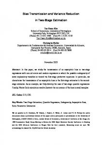
Figure 2: (a) A sample path Y of the M/M/1 queue with ρ = λ/µ = 0.9, and Y (0) = 400. (b) A solution to the differential equation φ˙ = I(φ > 0)(λ − µ) starting from the same initial condition. To construct an approximation to the solution to Poisson’s equation, first note that in heavy traffic, the network will typically be somewhat congested, and so we are primarily 19

concerned with “large” states. So it may pay to consider the process starting from a large initial condition. In the left-hand side of Figure 2 we see one such simulation. One approach to computing the solution to Poisson’s equation is to compute (15). While this is easy for the M/M/1 queue, such computation can be formidable for more complex network models. However, consider the right-hand side of Figure 2 which shows a sample path of the deterministic fluid, or leaky bucket model. This satisfies the differential equation φ˙ = I(φ > 0)(λ − µ), where I(·) is the indicator function that is 1 if its argument is true and 0 otherwise. The behavior of the two processes looks similar when viewed on this large spatial/temporal scale. It appears that a good approximation is h ∗ (x) ≈ Z ∞ ∆ φ(t) dt, φ(0) = x, h(x) = 0

=

1 x2 . 2µ−λ

(16)

This is the same approximation arrived at in Section 3. Of course, the M/M/1 queue is a very special case of a multiclass queueing network, and so it is worthwhile investigating this approximation more carefully before adopting it wholesale. We return now to the case of a general multiclass queueing network. The dynamics of the process Y can be described by a random linear system after a slight extension of the previous definitions. Define a sequence of i.i.d. random matrices P P 2 {I(n) : n ≥ 1} on {0, 1}(`+1) , with P{ j k Ij,k (n) = 1} = 1, and E[Ij,k (n)] = µj Rjk , where µj denotes the service rate for class j customers. Note that exactly one element of

I(n) is positive for each n. These random variables indicate which event in the uniformized process Y = (Y (n) : n ≥ 0) is to occur. The variable Ijk (n) = 1 if and only if a class j job completes service and moves to station k. It is convenient to capture the exogenous arrival processes within the same framework. An exogenous arrival is indicated by j = 0, and a ∆ P departure from the system is indicated by k = 0. For j = 0, let µ0 = `k=1 λk denote the overall arrival rate of customers to the system. Define R0,0 = 0, and for 1 ≤ k ≤ `,

R0,k = λk /µ0 . Thus, we pool all customer arrivals into one stream with rate µ0 , and an arriving customer is allocated to one of the ` classes according to the appropriate probability. For 1 ≤ j ≤ `, let Wj (n) = 1 if station s(j) is allocating its entire effort to customers 20

of class j at time n and 0 otherwise. As before we require that Wj (n) is a deterministic function of Y (n) for all n ≥ 0 and all j = 1, . . . , `. We define W0 (n) = 1 for all n, indicating that the exogenous arrival process is always active. For 1 ≤ k ≤ `, let e k denote ∆

the kth basis vector in R` , and set e0 = 0. The random linear system can then be defined as Y (n + 1) = Y (n) +

` ` X X

Ij,k (n + 1)[−ej + ek ]Wj (n),

(17)

j=0 k=0

where the state process Y denotes the vector of customer classes in the system as before. To define the fluid model associated with this network we suppose that the initial condition is large so that m = |Y (0)| À 1. We then construct a continuous time process φy (t) as follows: If tm is an integer, we set φy (t) =

1 Y (mt), m

where Y (0) = y and |y| = m. For all other t ≥ 0, we define φy (t) by linear interpolation, so that it is continuous and piecewise linear in t. Note that |φy (0)| = 1, and that φy is Lipschitz continuous. (See, e.g., Apostol [1969, p. 229] for a definition of Lipschitz continuity.) The collection of all “fluid limits” is defined by ∆

L=

∞ \

{φy : |y| > m}

m=1

where the overbar denotes weak closure. The set L depends upon the particular policy chosen, and for many policies such as preemptive priority policies, it is a family of purely deterministic functions. Any process φ ∈ L evolves on the state space R`+ and, for a wide class of scheduling policies, satisfies a differential equation of the form `

`

XX d φ(t) = µj Rjk [−ej + ek ]uj (t) dt

(18)

j=0 k=0

where the function u(·) is analogous to the discrete control, and satisfies similar constraints (see the M/M/1 queue model described earlier, or Dai [1995], Dai and Weiss [1996] for more general examples). In many cases the differential equation (18) admits a unique solution, from any initial condition, even though typically in practice the control u is a discontinuous function of the state φ (consider again any priority policy). 21

It is now known that stability of (17) is closely connected with the stability of the fluid model [Dai, 1995, Kumar and Meyn, 1996, Dai and Meyn, 1995]. The fluid model L is called Lp -stable if lim sup E[|φ(t)|p ] = 0.

t→∞ φ∈L

Let T0 denote the first hitting time inf{t ≥ 0 : φ(t) = 0}. It is shown in Meyn [1997] that supφ∈L E[T0 ] < ∞ when the model is L2 -stable. Hence, when L is non-random, L2 stability is equivalent to stability in the sense of Dai [1995]: There is some time T such that φ(t) = 0 for t ≥ T , φ ∈ L. For example, in the M/M/1 queue with λ < µ, the queue eventually hits 0 as seen in Figure 2. The following result is a minor generalization of results from Kumar and Meyn [1996], Dai and Meyn [1995]. Its proof is omitted. Theorem 3 The following two stability criteria are equivalent for the network under any non-idling policy, and any p ≥ 2. (i) There is a function V , and a constant b < ∞ satisfying P V (y) − V (y) ≤ −|y|p−1 + b where for some δ > 0, δ(1 + |y|p ) ≤ V (y) ≤ δ −1 (1 + |y|p ),

y ∈ S.

(19)

(ii) The fluid model L is Lp -stable.

Thus, Lp stability can be verified through the Lyapunov condition (A). Using this result it is possible to show that the solution to Poisson’s equation is asymptotically equal to a value function for the associated fluid model, provided that the fluid model is L 2 stable. It can be shown that many policies for the fluid model are piecewise constant on a finite set of cones in IR`+ . This is certainly the case for buffer priority policies, and also holds for L1 optimal policies (for a discussion see Weiss [1995]). It then follows that for such policies the fluid value function V is piecewise quadratic. The proof of the following result appears in the appendix. 22

Theorem 4 Suppose that for a given non-idling policy w, the fluid model L is L 2 -stable and non-random. Suppose moreover that limits are unique, in the sense that φ 1 (0) 6= φ2 (0) for any two distinct φi ∈ L. Then a solution h∗ to Poisson’s equation exists, and ¯ h∗ (y) ¯ ¯ ¯ lim sup¯ − 1¯ = 0, |y|→∞ V (y)

where

V (y) = |y|

2

Z

∞

|φ(t)| dt,

φ(0) =

0

y . |y|

Hence, under the conditions of Theorem 4, a solution h to Poisson’s equation is intimately related to the fluid value function V . This result then strongly motivates the use of a fluid value function as an approximation for the solution to Poisson’s equation. Another way to motivate the fluid approximation is to note that (from (17)) Y (n + 1) = Y (n) +

X

µj Rjk (−ej + ek )Wj (n)

j,k

+

X

(Ijk (n + 1) − µj Rjk )(−ej + ek )Wj (n)

j,k

= Y (n) + BW (n) + D(n + 1) n X = Y (0) + BW (i) + M (n + 1),

(20)

i=0

where B is an (` + 1) × (` + 1) matrix. The process M (·) is a vector-valued martingale with respect to the natural filtration, and D(i) is the martingale difference M (i) − M (i − 1). (See, e.g., Ross [1996] for an introduction to martingales.) It is straightforward to check that ED(i)0 D(i) is bounded in i (by b say), so that EM (n)0 M (n) ≤ bn for all n ≥ 0. Hence, the network is essentially a deterministic fluid model with a ‘disturbance’ M . When the initial condition Y (0) is large, then the state dominates this disturbance, and hence the network behavior appears deterministic. We therefore have strong motivation for approximating the solution to Poisson’s equation h∗ by V , where 4

V (y) =

Z

∞

φ(t) dt, 0

23

and φ solves the differential equation (18) with φ(0) = y. The fluid estimator of α is then n−1

βX ∆V (Y (k)). αf (n) = |Y¯ (n)| + n

(21)

k=0

The parameter β is again a constant that may be chosen to attempt to minimize the variance of the fluid estimator. We use the methodology outlined in the appendix to estimate the optimal β. Consequently, the asymptotic results for the quadratic estimator also apply here, namely that under the assumption (A), the fluid estimator is weakly consistent, and is asymptotically t-distributed when suitably normalized. Clearly, to implement the fluid estimator we need to be able to compute ∆V . For any function V , we have that P V (y) = Ey V (Y (1)) =

` ` X X

µj Rjk V (y − ej + ek )Wj (y),

j=0 k=0

so that it suffices to be able to compute V (y) for y ∈ S. Solving the differential equation (18) to find φ is not difficult when the fluid control u is piecewise constant on a finite set of cones in IR`+ since in this case φ is piecewise linear. Integrating φ to find the fluid value function V is then straightforward. In other words, for a specific model, some preliminary work has to be done to give code that can compute V , but this is usually not a difficult step. Algorithms for computation or approximation of V are described in Eng and Meyn [1996], Borkar and Meyn [2003]. It should be apparent from the above discussion that computing the control ∆ V for the estimator (21) may be moderately time-consuming (computationally speaking) relative to the time taken to simply simulate the process Y . Be that as it may, it is certainly the case that the time taken to compute the control is relatively insensitive to the congestion in the system. In Table 3 we present simulation results for the fluid estimator on the network of Figure 1. (Similar results were obtained for all other multiclass queueing networks that we tried.) The entries in Table 3 have the same interpretation as those in Table 1. In particular, the column headed “Reduction” represents the variance reduction factor over the standard estimator. 24

Table 3: Simulation results for the two-station three-buffer example (2 significant figures). The interpretation of the values given is the same as in Table 1. ρ2

Mean

Var

Reduction

0.2

0.47

6.1E-5

3.5

0.4

1.3

4.0E-4

3.5

0.6

2.8

3.5E-3

3.1

0.8

6.9

4.3E-2

4.4

0.9

14

0.17

12

0.95

26

0.23

56

0.99

110

0.98

100

The best value of β was found to be close to unity in each of the simulations, particularly at high loads where it was found to be within ±5% of unity. Observe that for low traffic intensities, the fluid estimator yields reasonable variance reductions over the standard estimator. However, because it is more expensive to compute than the standard estimator, these results are not particularly encouraging. But as the system becomes more and more congested, the fluid estimator yields large variance reductions over the standard estimator, meaning that the extra computational effort per iteration is certainly worthwhile. For very high traffic intensities, the fluid estimator is significantly outperforming both the standard estimator and the quadratic estimator, and so we have achieved our goal of deriving an estimator that can be effective in heavy traffic.

5

Conclusions

We have given two simulation estimators for estimating a linear function of the steadystate customer class population. The quadratic estimator produces very useful variance reductions in light to moderate traffic at very little additional computational cost. We recommend that it be used in simulations of such lightly-loaded networks. The quadratic estimator is less effective

25

in simulations of heavily-loaded networks, but could potentially provide useful variance reductions in this regime if a better choice of weighting vector ν can be employed. The fluid estimator provides modest variance reduction in light to moderate traffic, but appears to be very effective in heavy traffic. There is an additional computational overhead in computing the fluid estimator, but this overhead is (roughly) independent of the load on the network. Hence we may conclude that in heavily-loaded systems, the fluid estimator should yield significant computational improvements, and should therefore be used. One might conclude from the above discussion that the quadratic and fluid estimators could be combined using the method of multiple control variates to yield a single “combined” estimator. However, we believe that it is unlikely that a combined estimator would yield significant improvements over the use of either the quadratic estimator (in light traffic) or the fluid estimator (in heavy traffic). In light traffic, we expect that the additional reductions in variance would be negated by the increased computational effort. And in heavy traffic we expect that any additional variance reduction would be modest, owing to the weaker performance of the quadratic estimator in this regime.

Appendix Proof of Theorem 2 It is straightforward to show that ∆f 2 (y) = −2(1 − ρ)f (y) + e0 Q[Λ + Q−1 W − M W R + diag(e0 M W R)]Q0 e,

(22)

where W is the diagonal matrix containing the work allocation vector w corresponding to y, and Λ =diag(λ). Furthermore, for m ≥ 3, ∆f m (y) = −m(1 − ρ)f m−1 (y) + lower order terms.

(23)

It follows from (23) with m = 5 that (A) holds. This implies (Theorem 17.5.3 of Meyn and Tweedie [1993]) that the TAVC’s are finite, and furthermore, that σf2 (ρ) = lim n Var(d0 Y¯ (n)), and n→∞

26

σi2 (ρ) = lim n Var(Y¯i (n)). n→∞

The fact that h is of the form given in the theorem follows from (22). Observe that the function f 2 /(2(1 − ρ)) is “almost” the solution to Poisson’s equation. It needs to be adjusted slightly to remove the terms in the RHS of (22) involving the work allocation vector w. These terms are of the form f 0 w, where the coefficients in f are bounded in ρ. Therefore, the solution to Poisson’s equation is as given in the Theorem. So then the TAVC σf2 (ρ) is given by E h(Y )(f (Y ) − d0 y¯) =

Cov(f 2 (Y ), f (Y )) − E(c0ρ Y (f (Y ) − d0 y¯)), 2(1 − ρ)

(24)

where Y is distributed according to the stationary distribution π and y¯ = E Y . Since E ∆f m (Y ) = 0 for m = 0, . . . , 4, it follows from (22) that E f (Y ) is of the order (1 − ρ)−1 as ρ → 1. Then, by induction using (23), E f m (Y ) is of the order (1 − ρ)−m as ρ → 1 for m = 1, . . . , 4. The second term on the right-hand side of (24) is therefore of the order (1 − ρ) −3 as ρ → 1. As for the first term, we have the easily-proved inequality that for any non-negative r.v. X with E X 3 < ∞, Cov(X 2 , X) ≥

Var X E X 3. E X2

Applying this inequality to the first term on the right-hand side of (24), and noting that Var f (Y ) is of the same order as E f (Y )2 as ρ → 1, we obtain the required result that σf2 (ρ) is of the order (1 − ρ)−4 as ρ → 1. The last statement of the theorem follows from the fact that σf2 (ρ) = =

≤

lim n Var(d0 Y¯ (n))

n→∞

lim n Var(

n→∞

lim `n

= `

di Y¯i (n))

i=1

n→∞

` X

` X

` X

Var(di Y¯i (n))

i=1

d2i σi2 (ρ).

i=1

27

Control Variates in Steady-State Simulation We repeat formulae (given in Loh [1994]) for estimating the control variate parameter β that is used in both the quadratic estimator (12) and the fluid estimator (21) using the batch means method of simulation output analysis. To encapsulate both estimators and avoid repetition, we give the formulae for the case where a real-valued stochastic process X = (X(n) : n ≥ 0) is simulated, and a real-valued control C = (C(n) : n ≥ 0) is recorded. Let the b batches each consist of m observations, so that the simulation run-length n = mb. If Xi and Ci are the ith batch means of the process and control respectively, then for 0 ≤ i ≤ b − 1, we have 1 Xi = m

(i+1)m−1

X

j=im

1 X(j) and Ci = m

(i+1)m−1

X

C(j).

j=im

¯ n and C¯n denote the overall (sample) means of the process and control respectively. Let X Define b−1

VXX (n) = VCC (n) = VXC (n) =

1 X ¯ n )2 , (Xi − X b−1 1 b−1 1 b−1

i=0 b−1 X i=0 b−1 X

(Ci − C¯n )2 , and ¯ n )(Ci − C¯n ). (Xi − X

i=0

¯ n + β C¯n be the controlled estimator. Define β = −VXC /VCC , and let αn = X Finally, let b−1 R (n) = b−2 2

µ ¶ VXC (n)2 VXX (n) − VCC (n)

and 2

2

S (n) = R (n)

µ

¶ 1 1 C¯n2 + . b b − 1 VCC

(25)

Using the above computational process, we can construct the quadratic estimator α q (n) and the fluid estimator αf (n). The following result describes the asymptotic behavior of these estimators.

28

Theorem 5 (Loh 1994) Under the assumption (A), the estimators αq (n) and αf (n) converge in probability to α, and for j = q, f , αj (n) − α ⇒ Tb−2 , Sj (n) where Tb−2 has the Student’s t-distribution with b − 2 degrees of freedom, and Sj (n) is defined in the obvious way through (25). Proof. The second result is proved in Section 1.3.2 of Loh [1994]. In addition, Proposition 1.5 of Loh [1994] shows that nSj2 (n) converges in distribution to a finite-valued random variable as n → ∞ so that the first result follows.

5.1

Proof of Theorem 4

First note that for any φ ∈ L we have |φ(0)| = 1, and under the assumptions of the theorem there is a T > 0 such that Z T V (y) = |y|2 |φ(t)| dt,

φ(0) =

0

y , |y|

φ ∈ L.

We shall fix such a T throughout the proof. From Theorem 3, a Lyapunov function exists that satisfies (4) which is equivalent to a quadratic in the sense of (19). It follows that π(c) < ∞, where c(y) = |y|, and that a solution to Poisson’s equation exists which is bounded from above by a quadratic, and uniformly bounded from below [Meyn and Tweedie, 1993, p. 432]. We can then take the solution to Poisson’s equation and iterate as follows: P n h = P i ¯, where c ¯(y) = |y| − α. Let m = |y| and take n = [mT ] = the integer part of h − n−1 i=0 P c mT to give

Ey [h(Y (mT ))] h(y) = − 2 m m2

Ey

hP

mT −1 |Y (i)| i=0 m

m

i

−

Tα . m

Since h is bounded above by a quadratic, there is a K < ∞ such that ¯ ¯ ³ 2´ ¯ [h(Y (mT ))] ¯ ¯ ¯ ≤ K 1 + |Y (mT )| ¯ ¯ m2 m2

The random variable on the right hand side is uniformly bounded by K(1 + 1/m + T ) 2 for all initial y since at most one customer can arrive during each time slot. It then follows 29

from weak convergence and the definition of T that ¯ ¯ ¯ [h(Y (mT ))] ¯ ¯ ¯=0 lim sup Ey ¯ ¯ 2 m |y|→∞

Moreover, again by Lipschitz continuity of the fluid model we have ¯ ¯ " mT −1 # ¯ y ¯¯ 1 X |Y (i)| ¯ − V ( )¯ = 0. lim sup ¯Ey m m m ¯ |y|→∞ ¯ i=0

Putting these results together we see that ¯ ¯ ¯ h(y) y ¯¯ ¯ lim sup ¯ 2 − V ( )¯ = 0, m m |y|→∞

proving the result.

References T. M. Apostol. Calculus, Volume 2. Wiley, New York, 2nd edition, 1969. S. Asmussen. Queueing simulation in heavy traffic. Mathematics of Operations Research, 17:84–111, 1992. F. Baskett, K. M. Chandy, R. R. Muntz, and F. G. Palacios. Open, closed, and mixed networks of queues with different classes of customers. Journal of the ACM, 22:248–260, 1975. D. Bertsekas and R. Gallagher. Data Networks. Prentice Hall, Englewood Cliffs, NJ, 1987. D. Bertsimas, I. Paschalidis, and J. N. Tsitsiklis. Optimization of multiclass queueing networks: polyhedral and nonlinear characterizations of achievable performance. Ann. Appl. Probab., 4:43–75, 1994. V. S. Borkar and S. P. Meyn. Value functions and performance evaluation in stochastic network models. 42nd IEEE Conference on Decision and Control,December 9-12, 2003 Hyatt Regency Maui, Hawaii, USA (submitted), 2003. J. A. Buzacott and J. G. Shanthikumar. Stochastic Models of Manufacturing Systems. Prentice Hall, Englewood Cliffs, NJ, 1993. 30

J. G. Dai. On positive Harris recurrence of multiclass queueing networks: a unified approach via fluid limit models. Ann. Appl. Probab., 5(1):49–77, 1995. J. G. Dai and J. M. Harrison. Reflected Brownian motion in an orthant: numerical methods for steady-state analysis. Ann. Appl. Probab., 2(1):65–86, 1992. J. G. Dai and S. P. Meyn. Stability and convergence of moments for multiclass queueing networks via fluid limit models. IEEE Transactions on Automatic Control, 40:1889– 1904, 1995. J. G. Dai and G. E. Weiss. Stability and instability of fluid models for reentrant lines. Math. Operations Res., 21:115–134, 1996. D. G. Down and S. P. Meyn. Piecewise linear test functions for stability of queueing networks. In Proceedings of the 33rd Conference on Decision and Control, pages 2069– 2074, Buena Vista, FL, December 1994. J. Eng, D. Humphrey and S. P. Meyn. Fluid network models: Linear programs for control and performance bounds. In J. C. J. Gertler and M. Peshkin, editors, Proceedings of the 13th IFAC World Congress, volume B, pages 19–24, San Francisco, California, 1996. S. B. Gershwin. Manufacturing Systems Engineering. Prentice Hall, Englewood Cliffs, NJ, 1993. P. W. Glynn and W. Whitt. The asymptotic efficiency of simulation estimators. Operations Research, 40:505–520, 1992. J. M. Harrison and R. J. Williams. Multidimensional reflected Brownian motions having exponential stationary distributions. Ann. Probab., 15(1):115–137, 1987. J. M. Harrison and R. J. Williams. On the quasireversibility of a multiclass Brownian service station. Ann. Probab., 18(3):1249–1268, 1990. S. Henderson. Variance Reduction Via an Approximating Markov Process. PhD thesis, Department of Operations Research, Stanford University, Stanford, California, USA, 1997. 31

S. Henderson, S. P. Meyn, and V. Tadic. Performance evaluation and policy selection in multiclass networks. Discrete Event Dynamic Systems, 13:149–189, 2003. Special issue on learning and optimization methods. S. G. Henderson and P. W. Glynn. Approximating martingales for variance reduction in Markov process simulation. Mathematics of Operations Research, 27:253–271, 2002. S. G. Henderson and S. P. Meyn. Efficient simulation of multiclass queueing networks. In S. Andradottir, K. J. Healy, D. H. Withers, and B. L. Nelson, editors, Proceedings of the 1997 Winter Simulation Conference, pages 216–223, Piscataway NJ, 1997. IEEE. J. R. Jackson. Jobshop-like queueing systems. Management Science, 10:131–142, 1963. F. P. Kelly. Reversibility and Stochastic Networks. Wiley, New York, NY, 1979. P. R. Kumar and S. P. Meyn. Duality and linear programs for stability and performance analysis queueing networks and scheduling policies. IEEE Transactions on Automatic Control, 41(1):4–17, 1996. S. Kumar and P. R. Kumar. Performance bounds for queueing networks and scheduling policies. IEEE Transactions on Automatic Control, 39:1600–1611, 1994. S. Lavenberg. Computer Performance Modeling Handbook. Academic Press, New York, NY, 1983. S. S. Lavenberg and P. D. Welch. A perspective on the use of control variables to increase the efficiency of Monte Carlo simulations. Management Science, 27:322–335, 1981. A. M. Law and W. D. Kelton. Simulation Modeling and Analysis. McGraw-Hill, New York, 3rd edition, 2000. W. W. Loh. On the Method of Control Variates. PhD thesis, Department of Operations Research, Stanford University, Stanford, CA, 1994. S. P. Meyn. Stability and optimization of queueing networks and their fluid models. In Mathematics of Stochastic Manufacturing Systems (Williamsburg, VA, 1996), pages 175–199. Amer. Math. Soc., Providence, RI, 1997. 32

S. P. Meyn. Sequencing and routing in multiclass queueing networks. Part I: Feedback regulation. SIAM J. Control Optim., 40(3):741–776, 2001. S. P. Meyn and R. L. Tweedie. Markov Chains and Stochastic Stability. Springer-Verlag, London, 1993. J. R. Morrison and P. R. Kumar. New linear program performance bounds for queueing networks. Journal of Optimization Theory and Applications, 100:575–597, 1999. B. L. Nelson. Control variate remedies. Operations Research, 38:974–992, 1990. M. F. Neuts. Matrix-Geometric Solutions in Stochastic Models. Dover Publications Inc., New York, 1994. An Algorithmic Approach, Corrected reprint of the 1981 original. S. M. Ross. Stochastic Processes. Wiley, New York, 2nd edition, 1996. P. J. Schweitzer. Aggregation methods for large Markov chains. In Mathematical Computer Performance and Reliability (Pisa, 1983), pages 275–286. North-Holland, Amsterdam, 1984. E. Schwerer. A linear programming approach to the steady-state analysis of reflected Brownian motion. Stochastic Models, 17:341–368, 2001. X. Shen, H. Chen, J. G. Dai, and W. Dai. The finite element method for computing the stationary distribution of an SRBM in a hypercube with applications to finite buffer queueing networks. Queueing Systems, 42(1):33–62, 2002. G. Weiss. Optimal draining of a fluid re-entrant line. In F. Kelly and R. Williams, editors, Volume 71 of IMA volumes in Mathematics and its Applications, pages 91–103, New York, 1995. Springer-Verlag. W. Whitt. Planning queueing simulations. Management Science, 35:1341–1366, 1989.

33