Ensemble of Specialized Neural Networks for Time Series Forecasting Slawek Smyl –
[email protected] ISF 2017
Ensemble of Predictors • Ensembling a group predictors (preferably diverse) or choosing one of them do a forecast in a particular situation is an attractive idea being actively researched. • Dr. Sven F. Crone in his talk* during 2016 International Joint Conference on Neural Networks (IJCNN) reported a method of creating diversity of a group of neural networks by training them on different subset of features. • My work has been inspired by his talk, but it uses different method of achieving the diversity and also attempts a more traditional (and usually unsuccessful goal J) of choosing a best predictor from a pool. *Sven F. Crone and Stephan Häger, Feature selection of autoregressive Neural Network inputs for trend Time Series Forecasting , 2016 International Joint Conference on Neural Networks (IJCNN)
The Idea 1. Create a pool of NNs that specialize (i.e. are particularly good) in a subset of time series. 2. Find a good way either to ensemble them or to choose one of them to do the forecast • An obvious way to approach task 1 is to apply clustering, but it is not obvious what metric should be used, as a standard metric may not have much to do with the forecasting performance
Data Preprocessing
All experiments were done on 1428 monthly time series of M3 Competition data set (package Mcomp of R)
Data Preprocessing, cont. All inputs and outputs are normalized (e.g. divided) by some reasonably stable value reflecting size of the series near end of the output window. Here it is last point of deseasonalized and smoothed input
Data Preprocessing, cont. This is a simple data processing. Instead we could e.g. 1. Create several (perhaps overlapping) smaller output windows 2. Apply statistical algorithm on the time series (up to and including last input point) and extract some features (e.g. acf, ETS model types, ETS forecast)
Data Preprocessing, cont. Last record in the training set (for this time series)
Data Preprocessing, cont. Last record (and only one used) in the validation set (for this time series)
Because M3 time series are short, each of them is split into training part, and an nonoverlapping validation part composed of last 18 points (=forecast horizon). I am not doing a proper backtesting.
Neural Network Architecture Output (vector of max forecast horizon length)
Standard hidden layer (no bias)
LSTM2
LSTM1
Inputs
• Applying idea of ResNet (Residual Networks) while stacking LSTM (Long Short Term Memory) recurrent neural networks
Loss Function • Many Neural Network systems allow to specify a custom loss function, which opens possibility to • Optimize for a metric (e.g. sMAPE) • Using pinball loss to make a neural network to do a quantile regression, and therefore by running it several times getting a number of prediction intervals.
E.g. in CNTK, using Python, one can define sMAPE loss as def sMAPELoss (z, t): loss=o.reduce_mean(o.abs(t-z)/(t+z))*200 return loss
This definition will work, even if actuals and forecasts are normalized by dividing by a common ‘level’
Task 1: Creating Pool of Specialized NNs • Start with randomly allocating a part, e.g. half of the time series, to each network (e.g. 7 of them) • In a loop for each network • Execute a single training on the allocated training subset • Record performance on the whole training set (insample, average per all points of the training part of a series) • Rank the networks for each series. A series gets allocated to top N (e.g. 2) best networks • Repeat, make an early stop when average error in the validation area starts growing.
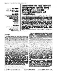
An example allocation of 10 series to 7 nets, topN=2 6 5 4 3 2 1 0 Net1
Net2
Net3
Net4
Net5
Net6
Net7
Series 1
Series 2
Series 3
Series 4
Series 5
Series 6
Series 7
Series 8
Series 9
Series 10
Task 1: Creating Poll of Specialized NNs, cont. • The success is reinforced – a network that does well, on average, with a particular series is likely to see it again in the next epoch of training, and will surely see it if this network is the best on it. • The experiments were done with recurrent NNs, therefore a particular net was receiving the whole series. If I were to use standard networks, without state, it would be possible to allocate pieces of one series to different networks. • The architecture, inputs are all the same, what is different, and actively manipulated between epochs, is the composition of the training data set for each network.
Example: Identity of best network for a particular series along the series steps: [ 0., 0., 1., 0., 0., 0., 0.] [ 0., 1., 0., 0., 0., 0., 0.] [ 0., 1., 0., 0., 0., 0., 0.] [ 0., 0., 0., 0., 0., 0., 1.] [ 0., 0., 0., 0., 0., 0., 1.] [ 0., 0., 0., 0., 0., 0., 1.] [ 0., 0., 0., 0., 0., 0., 1.] [ 0., 0., 0., 0., 0., 0., 1.] [ 0., 0., 0., 0., 0., 0., 1.] [ 0., 0., 0., 0., 0., 0., 1.] [ 0., 0., 0., 0., 0., 0., 1.] [ 0., 0., 0., 0., 0., 0., 1.]
Task 2: Ensembling or Choosing Best Network • Advanced, second-level network methods
• Using forecasts of each of the network as an additional input to the final network - did not work • Creating a recommender network that chooses which of the base network should deal with a particular forecast – did not work • Creating a network that outputs weights for the base network – did not work
• Simpler, rule methods worked • • • • • •
Simple average Weighted average by average training loss Weighted average by average frequency of being a best network Weighted average of top N (2) networks (average loss in training) Choosing a network that was best on the last training point Choosing a network that was best on average
Comparing Network – Validation Results, sMAPE Specialized
Non-specialized
Best Possible (perfect choosing of) single net
11.46
13.47
Single net
14.15, sd=0.06
14.37, sd=0.04
Best nets (min avg error over all training points of a series) Single best (best at last training point) net
14.51, sd=0.07
Ensemble of top 2 out of 7 nets (by average error over all training points of a series)
14.09, sd=0.04
Weighted ensemble of the above nets
13.99
14.3
14.35
Results In Context M3 dataset is a popular dataset, sMAPE, Monthly series: ARIMA
14.98
Ensemble of non-specialized NNs
14.35
ETS (ZZZ)
14.15
Ensemble of specialized NNs
13.99
Hybrid (mean of ARIMA and ETS)
13.91
Best algorithm in M3 competition
13.89 (THETA)
SGT
13.72, sd=0.019
Best of Bagged ETS
13.64 (BLD.MBB)
SGT – Seasonal, Global Trend is my algorithm that is a kind of generalized Exponential Smoothing, it has generalized (between additive and multiplicative) trend, Student distribution of error, a function for error size etc., fitted with MCMC.
Questions? Slawek Smyl –
[email protected]
Tools Used - CNTK • Microsoft’s CNTK, which used to mean Computational Network Toolkit, but now it means Cognitive Toolkit J • It is modern, fast and, I believe, easier to use than Tensorflow. • Open sourced, it runs on Windows and Linux. • It has own scripting/configuration language, as well as Python APIs that I used. Also C++ and some C# APIs.
SGT – Seasonal Global Trend Algorithm • Created by S. Smyl time series algorithm that generalizes (between additive and multiplicative) Trend and Error Exponential Smoothing models. • It uses Student-t distribution for errors • Formula for the expected value: µt =(𝑙#$%+𝛾 ∗ 𝑙#$%) ) ∗ 𝑠# where 𝑙#$% is previous level; γ is the global trend coefficient; 𝑝 ∈
• Function for scale of the error distribution: σ ∗ 𝑙#$%0 + 𝜍 where σ, 𝜍 are positive, and 𝜏 ∈
• All parameters are fitted by MCMC (Stan)
LGT – Local Global Trend Algorithm • Created by S. Smyl time series algorithm that generalizes Additive and Multiplicative Trend and Error Exponential Smoothing models. • It uses Student-t distribution for errors • Formula for the expected value: µt = 𝑙#$% + γ ∗ 𝑙#$%3 + λ ∗ 𝑏#$% where 𝑙#$% is previous level; γ is the global trend coefficient; 𝑝, λ ∈ ; 𝑏#$% is previous (local) trend
• Function for scale of the error distribution: σ ∗ 𝑙#$%0 + 𝜍 where σ, 𝜍 are positive, and 𝜏 ∈
• All parameters are fitted by MCMC (Stan)
My ISF 2016 paper: Results for Yearly M3 series Algorithm/Metric ETS (ZZZ) ARIMA Auto NN (M3 participant)
sMAPE 17.37 17.12 18.57
MASE 2.86 2.96 3.06
Best algorithm in M3
16.42 (RBF)
2.63 (ROBUST-Trend)
LSTM with minimal 16.4 preprocessing
2.88
LSTM using ETS for 15.94 preprocessing
2.73
LSTM using LGT for 15.46 preprocessing
2.65
LGT
2.50, sd= 0.004
15.23, sd= 0.015
• 645 series (rather short, 14-40 points) 200 B 𝑦# − 𝑦A# 𝑠𝑀𝐴𝑃𝐸 = > ℎ A# #C% 𝑦# + 𝑦 𝑀𝐴𝑆𝐸 =
ℎ$% ∑B#C% 𝑦# − 𝑦A# F𝑛 − 𝑠)$% ∑J0CHK% 𝑦0 − 𝑦I 0$H
Summation happens over prediction horizons, except for the divisor of the MASE equation, where it happens over past (in-sample) data
Quantile Regression and Pinball Loss • In “normal” regression we minimize sum of squared errors, that leads to average value forecast . • If we minimize L1 metric, we get median forecast. • More generally, if we minimize Pinball loss defined as (Forecast-Actual)*tau when Forecast>Actual (Actual-Forecast)*(1-tau) otherwise we are going to obtain quantile forecast for the specified quantile value, tau, e.g. 0.95 Code for Pinball loss in CNTK:
def PinballLoss (z, t, tau): tauV=o.constant(tau, shape=t.shape, dtype=np.float32) tau1mV=o.constant(1-tau, shape=t.shape, dtype=np.float32) loss=o.reduce_mean(o.element_select(o.greater_equal(t, z o.element_times(o.minus(t,z tauV o.element_times(o.minus(z,t tau1mV))) return loss