Oct 31, 2016 - The paper presents a novel algorithm for computing worst case execution time. (WCET) or maximum termination time of real-time systems ...
arXiv:1610.09795v1 [cs.FL] 31 Oct 2016
Finding Minimum and Maximum Termination Time of Timed Automata Models with Cyclic Behaviour Omar Al-Bataineh1 , Mark Reynolds2 , and Tim French2 1 Nanyang Technological University, Singapore 2 University of Western Australia, Australia
Abstract The paper presents a novel algorithm for computing worst case execution time (WCET) or maximum termination time of real-time systems using the timed automata (TA) model checking technology. The algorithm can work on any arbitrary diagonal-free TA and can handle more cases than previously existing algorithms for WCET computation, as it can handle cycles in TA and decide whether they lead to an infinite WCET. We show soundness of the proposed algorithm and study its complexity. To our knowledge, this is the first model checking algorithm that addresses comprehensively the WCET problem of systems with cyclic behaviour. In [BFH+ 01] Behrmann et al provide an algorithm for computing the minimum cost/time of reaching a goal state in priced timed automata (PTA). The algorithm has been implemented in the well-known model checking tool UPPAAL to compute the minimum time for termination of an automaton. However, we show that in certain circumstances, when infinite cycles exist, the algorithm implemented in UPPAAL may not terminate, and we provide examples which UPPAAL fails to verify.
1. Introduction In this paper, we consider the problem of computing the “worst case execution time” (WCET) in timed automata. Given a timed automaton A with a start location ls and a final location lf , this problem asks to compute an upper bound on the time needed to reach the final location lf from the start location ls . The problem is easy to solve in the case of acyclic TA [ABRF14], but cycles might introduce an unbounded WCET, that needs to be detected on-the-fly during the analysis. In general, WCET analysis is undecidable: it is undecidable to determine whether or not an execution of a system will eventually halt. However, for TA models one can use model-checking techniques to analyse the system and compute the WCET. Typically, the infinite state-space of a timed transition system is converted into an equivalent finite state-space of a symbolic transition system called a zone graph [Dil90, CGP01]. In a zone graph, zones (i.e. sets of valuations of the timed automaton clocks) are used to denote symbolic states. The zone graph Preprint submitted to Elsevier
Figure 1: A1 : an automaton with finite cycle
Figure 2: A2 : an automaton with infinite cycle
has been successfully used for the verification of safety and liveness properties of timed automata. Although the zone graph is precise enough to preserve the reachability properties in TA, it is too abstract to infer continuous time progress. At each step of the successor computation, the generated zones are extrapolated (abstracted) using a set of extrapolation operators and then canonicalized (tightened) in order to obtain a unique representation of the resulting zones. A test for inclusion of zones is then applied to check whether the new generated zone at a particular control location in the graph is already covered by some previously generated zones associated with that location. This helps to ensure termination of the analysis of TA even when infinite cycles exist. However, the classical abstraction used for verification of reachability problem [BY04] is not correct for WCET and BCET computation, as they give abstract zones and hence result in abstract values of the execution times. To demonstrate the problem, we give in Figures 1 and 2 two automata where both generate identical zone graphs when applying the standard zone approach for reachability analysis. The automaton A1 represents an automaton with finite cycle where WCET (A1 ) = 12. For this automaton, the standard zone approach can compute correctly the WCET without involving any extra check. On the other hand, the automaton A2 represents an automaton with an infinite cycle where WCET (A2 ) = ∞. For this automaton, the zone approach for reachability analysis fails to give the correct answer for WCET since it returns 12 instead of ∞. Note that if we disable extrapolation during the analysis, the search may not stop and we may not be able to obtain an answer. In a previous work [ABRF14], we proposed a zone-based solution to the problem of computing WCET of real-time systems modelled as TA. The proposed solution allows one to compute the WCET of TA in only one run of the zone construction instead of making repeated guesses (guided by binary search) and multiple model checking queries as done in [Met04]. However, in [ABRF14] we limit applicability of our solution to timed automata without infinite cycles. In the present paper, we give a more general solution to the problem that can
2
work on any arbitrary diagonal-free TA1 including those containing infinite cycles. Infinite cycles indeed make the computation of WCET difficult because zone extrapolation techniques are necessary to compute a finite state-space, and extrapolation prevents a straightforward computation of the WCET. The main contribution of the paper is therefore to propose an extrapolation technique that is compatible with the WCET computation. More precisely, we give the special conditions needed to define a forward zone-based reachability algorithm that terminates and computes the correct maximal time. Thus, the provided solution can be a significant break-through in computing WCET. The proposed extrapolation technique is an interesting addition to the collection of techniques for TA analysis. It is particularly useful because it improves zone extrapolation, that is one of the weak points of TA symbolic analysis. In [BFH+ 01] Behrmann et al propose an algorithm that aims to provide a solution to the minimum cost/time reachability problem in Uniformally Priced Timed Automata (UPTA) in the presence of extrapolation. The algorithm has been implemented in the well-known model checking tool UPPAAL to compute the minimum time for termination of an automaton. However, the extrapolation step is not detailed in [BFH+ 01] and the implementation in UPPAAL is often unable to terminate when the model has some cycles. The key difficulty in developing a solution to the minimum/maximum termination time problems using the zone approach is to define an abstraction of zones that guarantees termination of the algorithm, while keeping information precise for the extra clock that is used to compute the execution time of the automaton. This involves adapting two classical operations on zones: extrapolation and canonicalization. The later was forgotten in [BFH+ 01] leading to non termination. We give a number examples by which we demonstrate how and why existing algorithms for computing BCET and WCET fail (including the one being now used in the tool UPPAAL). Related Work. It is claimed in [Wil04] that model checking is inadequate for WCET analysis. However, in [Met04] Metzner showed that model checking can be used efficiently for WCET analysis. He used model checking to improve WCET analyses for hardware with caching. The use of timed automata (TA) and the model-checker UPPAAL for computing WCET on pipelined processors with caches was reported in [DOT+ 10] where the METAMOC method is described. METAMOC consists in: 1) computing the CFG of a program, 2) composing this CFG with a (network of timed automata) model of the processor and the caches. Computing the WCET is then reduced to computing the longest path (timewise) in the network of TA. The work in [BFH+ 01] uses a variant of timed automata called “Priced Timed Automata” and the DBM data structure to compute the minimum cost of reaching a goal state in the model. A priced timed automaton can associate 1 A class of TA in which the test of the form x − y ∼ c is disallowed, where x, y are clock variables, c is a constant, and ∼∈ {, ≥}.
3
costs with locations, where the costs are multiplied by the amount of time spent in a location. An automaton may be designed so that the total cost corresponds to the execution time, and thus this approach may be used to calculate the best case execution time problem. However, the WCET problem is different than the BCET problem and needs special treatment during the analysis in particular when there are cycles in the behaviour of TA. In [BLR05] Behrmann et al. provide zone-based algorithms for parameter synthesis for two strict forms of TCTL properties: (1) AF≤p φ and (2) AG(ψ ⇒ AF≤p φ). The first form can be used to calculate the WCET of the given TA model. However, none of these two forms can be used to directly calculate optimum time or BCET of the model. The algorithms require the user to have some prior knowledge about the behaviour of the given model in the sense that the user has to identify the set of goal states (e.g. final states) in order to use a TCTL formula for calculating WCET. Moreover, it is not clear to us how this approach can be used to handle TA with infinite cycles and whether it can detect the cases where the WCET is infinity. In [ABRF14] Al-Bataineh et al present a solution to the problems of computing the shortest and the longest time taken by a run of a timed automaton from an initial state to a final state. The solution is conceptually a marked improvement over some earlier work on the problems [Met04], in which repeated guesses (guided by binary search) and multiple model checking queries were effectively but inelegantly and less efficiently used; while in [ABRF14] only one run of the zone construction is sufficient to yield the answers. However, the authors of [ABRF14] limit applicability of their approach to timed automata without infinite runs. The efficient verification of WCET of timed automata models with cyclic behaviour requires to detect on-the-fly the existence of infinite zeno runs (i.e. runs in which time cannot diverge) and infinite non-zeno runs (i.e. runs in which time can diverge) in the behaviour of the automaton under analysis. This is necessary in order to guarantee termination of the analysis. Detection of infinite non-zeno runs was already addressed in [AD94]. Their approach works on the region graph, but for correctness reasons, it cannot be used on (abstract) zone graphs. The trick involving adding an extra clock for non-zenoness is discussed in [Tri99, Tri05, AM04]. The problem of checking existence of zeno runs was formulated as early as in [Tri99]. A bulk of the literature for this problem also directs to [GB07, CY92, RS12]. All of these solutions provide a sufficient-only condition for the absence of zeno runs. However, the purpose of our work is to present the special conditions needed to define a forward zone-based reachability algorithm that terminates and computes the correct maximal time while using the abstract zone graph, which requires to handle on-the-fly infinite zeno runs and infinite non-zeno runs. The structure of the paper is as follows. We begin in Section 2 by introducing the syntax and the semantics of TA and the syntax and the semantics of the zone graph. We then review the existing extrapolation procedures of TA and discuss their role in forward reachability algorithms. In Section 3, we discuss some interesting issues about the minimum cost reachability algorithm proposed 4
by Behrmann et al [BFH+ 01] and its implementation in UPPAAL. In Section 4, we introduce what we call partial extrapolation procedure of zones and prove its correctness. We also discuss cycles (loops) in TA and describe what we call fixed point abstraction to detect (on-the-fly) infinite cycles. In Section 5, we describe a model checking algorithm for computing WCET for the class of diagonal-free TA. In Section 6, we study the complexity of the algorithm. In Section 7, we describe an implementation of the algorithm using the model checker opaal and describe the associated verification results on a set of examples. Finally, in Section 8, we draw some conclusions and discuss future directions. 2. Preliminaries 2.1. Timed Automata Timed automata are an extension of the classical finite state automata with clock variables to model timing aspects [AD94]. Let X be a set of clock variables, the clock valuation v for the set X is a mapping from X to R+ where R+ denotes the set of non-negative real numbers. Definition 1. A timed automaton A is a tuple (Σ, L, L0 , LF , X, I, E), where • Σ is a finite set of actions. • L is a finite set of locations. • L0 ⊆ L is a finite set of initial or starting locations. • LF ⊆ L is a finite set of final locations. • X is a finite set of clocks. • I : L → C(X) is a mapping from locations to clock constraints, called the location invariant. • E ⊆ L × L × Σ × 2X × C(X) is a finite set of transitions. An edge ′ ′ (l, l , a, λ, φ) represents a transition from location l to location l after performing action a. The set λ ⊆ X gives the clocks to be reset with this transition, and φ is a clock constraint over X. The clock constraint φ can be of the form: φ ::= x ≺ c | φ1 ∧ φ2 , where x ∈ X, c ∈ N, and ≺∈ {, ≥}. We define the semantics of a timed automaton by an infinite labelled transition system. The states in this system are tuples (l, v), where l is the current location of the automaton, and v is a function that maps the clocks of the automaton to a non-negative real number. The initial states are of the form (l0 , v0 ) where l0 in L0 and the valuation v0 (x) = 0 for all x ∈ X. With each transition we associate a clock constraint called a guard and with each location we associate a clock constraint called its invariant. Transitions of an automaton may include clock resets and guards which give conditions on the interval in which a transition can be executed. 5
Definition 2. Transitions in timed automata are of two forms: 1. delay transitions that model the elapse of time while staying at some loδ cation: for a state (l, v) and a real-valued time increment δ ≥ 0, (l, v) − → ′ ′ (l, v + δ) if for all v with v ≤ v ≤ v + δ, the invariant I(l) holds. 2. action transitions that execute an edge of the automata: for a state (l, v) ′ ′ a and a transition (l, l , a, λ, φ) such that v |= φ, (l, v) − → (l , v[λ := 0]). So for an automaton to move from a location to another a delay transition d i ai −→. followed by an action transition must be performed. We write this as −→ Definition 3. A run of a timed automaton with an initial state (l0 , v0 ) over a timed trace ζ = (t1 , a1 ), (t2 , a2 ), ... is a sequence of transitions of the form. d1 a1
d2 a2
hl0 , v0 i −→−→ hl1 , v1 i −→−→ hl2 , v2 i, ... satisfying the condition ti = ti−1 + di for all i ≥ 1 and that l0 ∈ L0 . Since the locations of an automaton are decorated with a delay-quantity and that transitions between locations are instantaneous, the delay of a run is simply the sum of the delays spent in the visited locations. d1 a1
d2 a2
Definition 4. Let r = hl0 , v0 i −→−→ hl1 , v1 i −→−→ hlP 2 , v2 i, ... be a run in the set of runs R. The delay of r, delay(r), is the sum ni=1 di , where n can be infinity. Hence, the problem of computing the BCET and WCET of A can be formalized as follows. BCET (A) = inf (delay(r)) ∀r∈Rf
WCET (A) = sup (delay(r)) ∀r∈R f
where R is the set of runs in R that reach a final location. Of course, a valid WCET bound is [0, ∞], and WCET can be infinity if there is an infinite non-zeno run (an infinite run in which time can diverge) [BG06, G´om06]. This can happen if there is a reachable cycle that can be repeated infinitely often and that time can elapse between iterations. Definition 5. A cycle in a timed automaton is a finite sequence of edges where the source location of the first edge in the sequence is the target location of the last edge in the sequence. Let A = (Σ, L, L0 , LF , X, I, E) be a timed automaton and let m be a natural number such that m ≥ 1. We say that a sequence (e0 , e1 , ..., em−1 ) ∈ E m is a cycle if trg(ei ) = src(ei+1 ) for all 0 ≤ i < m − 1 and trg(em−1 ) = src(e0 ).
6
2.2. The Clock Zones and The Difference Bound Matrices The infinite state-space of a TA can be converted into an equivalent finite state-space of a symbolic transition system called a zone graph [Dil90, CGP01]. A state in a zone graph is a pair (l, Z), where l is a location in the TA model and Z is a clock zone that represents a set of clock valuations at l. Formally a clock zone is a conjunction of inequalities that compare either a clock value or the difference between two clock values to an integer. In order to have a unified form for clock zones we introduce a reference clock x0 to the set of clocks X in the analyzed model that is always zero. The general form of a clock zone can be described by the following formula. ^ (x0 = 0) ∧ ((xi − xj ) ≺ ci,j ) 0≤i6=j≤n
where xi , xj ∈ X, ci,j bounds the difference between them, and ≺∈ {≤, M (xi ), ∞ if −m0,i > M (xi ), ′ ′ (mi,j ; ≺i,j ) = ∞ if −m0,j > M (xj ), i 6= 0 (−M (x ), M (xj ), i = 0 j (m , ≺ ) otherwise. i,j i,j
Similarly, we can define the Extra+ LU (Z) ∞ ∞ ′ ′ (mi,j ; ≺i,j ) = ∞ (−U (xj ), L(xi ), if −m0,i > L(xi ), if −m0,j > U (xj ), i 6= 0 if −m0,j > U (xj ), i = 0 otherwise.
2.4. The Standard Zone-based Approach Before presenting our proposed solution to the WCET problem it is necessary first to summarise how the zone or DBM based successor computation can be performed. Let D be a DBM in canonical form. We want to compute the suc′ cessor of D w.r.t to a transition e = (l, l , a, λ, φ), let us denote it as succ(D, e). The clock zone succ(D, e) can be obtained using a number of elementary DBM operations which can be described as follows. 1. Let an arbitrary amount of time elapse on all clocks in D. In a DBM this means all elements Di,0 are set to ∞. We will use the operator ⇑ to denote the time elapse operation. 2. Take the intersection with the invariant of location l to find the set of possible clock assignments that still satisfy the invariant. 3. Take the intersection with the guard φ to find the clock assignments that are accepted by the transition. 4. Canonicalize the resulting DBM and check the consistency of the matrix. 5. Set all the clocks in λ that are reset by the transition to 0. ′ 6. Take the intersection with the location invariant of the target location l . 7. Canonicalize the resulting DBM. ′ 8. Extrapolate and canonicalize the resulting zone at the target location l and check the consistency of the matrix. Combining all of the above steps into one formula, we obtain ′
succ(D, e) = (Canon(Extra(Canon((Canon(((D⇑ ) ∧ I(l)) ∧ φ)[λ := 0]) ∧ I(l ))))) where Extra represents an extrapolation function that takes as input a DBM and returns the M -form of the matrix, while Canon represents a canonicalization function that takes as input a DBM and returns a canonicalized matrix in the sense that each atomic constraint in the matrix is in the tightest form, I(l) is the invariant at location l, and ⇑ denotes the elapse of time operation. Note that intersection does not preserve canonical form [BY04], so we should canonicalize (((D⇑ ) ∧ I(l)) ∧ φ) before resetting any clock (if any). Since after executing the transition e all the clocks in the automaton have to advance at the same rate. After applying the guard, the matrix must be checked for consistency. Checking the consistency of a DBM is done by computing the canonical form and then checking the diagonal for negative entries. The resulting zone at step ′ 5 needs to be intersected with the clock invariant at the target location l and extrapolating/canonicalization afterwards. This is necessary in order to ensure that the guard φ and the reset operation ([λ := 0]) implies the invariant at the target location. Before proceeding further let us review first the three elementary operations that are used to construct the zone graph of a given automaton, which are the intersection operation, the reset operation, and the delay operation or the elapse of time operation.
10
Definition 8. (The intersection operation). We define D = D1 ∧ D2 . Let 1 2 Di,j = (c1 , ≺1 ) and Di,j = (c2 , ≺2 ). Then Di,j = (min(c1 , c2 ), ≺) where ≺ is defined as follows. ≺1 if c1 < c2 , ≺ if c < c , 2 2 1 ≺= ≺1 if c1 = c2 ∧ ≺1 =≺2 , < if c1 = c2 ∧ ≺1 6=≺2 ,
As mentioned before intersection does not preserve canonical form and the best way to put the matrix back on canonical form is to use the Floyd-Warshall algorithm. However, the work in [ZLZ05] presents an algorithm that improves the canonicalization of the matrix after the intersection operation which has a time complexity of O(n2 ) Definition 9. (The delay operation). Elapsing time means that the upper bounds of the clocks are set to infinity. That is, after that operation ∀x∈X : x − x0 < ∞ holds. Let D′ = D ⇑, then: ( ′ (∞,