CIS 1066
1
On the Optimum Design of Fuzzy Logic Controller for Trajectory Tracking Using Evolutionary Algorithms H. N. Pishkenari, S. H. Mahboobi, and A. Meghdari Center of Excellence in Design, Robotics and Automation (CEDRA) School of Mechanical Engineering Sharif Univ. of Tech., Iran E-mail:
[email protected]
Abstract—Differential Evolution (DE) and Genetic Algorithms (GA) are population based search algorithms that come under the category of evolutionary optimization techniques. In the present study, these evolutionary methods have been utilized to conduct the optimum design of the fuzzy controller for mobile robot trajectory tracking. Comparison between their performances has also been conducted. In this paper we will present a fuzzy controller to the problem of mobile robot path tracking for the CEDRA rescue robot with a complicated kinematical model. After designing the fuzzy tracking controller, the membership functions will be optimized by evolutionary algorithms in order to obtain more acceptable results. Index Terms—Differential Evolution; Fuzzy Controller; Genetic Algorithm; Optimization; Trajectory Tracking.
T
I. INTRODUCTION
HE optimization of non-linear and sophisticated problems has been an interesting issue in science and technology [1]. In recent years, evolutionary algorithms have been applied to the solution of the above problems in many engineering applications. The best known algorithms in this category include Genetic Algorithms (GA), Evolutionary Programming (EP), Evolution Strategies (ES) and Genetic Programming (GP). There are some hybrid algorithms which blend features of these algorithms and are hard to classify. They have been referred as Evolutionary Computation (EC) methods [2]. In general, only the information related to objective function is required by EC methods. Differential Evolution (DE), developed by Price & Storn [3], is one of the best EC methods. This method provides one of the best algorithms for solving the real-valued function. DE has a very high convergence speed [4]. In the present study two evolutionary methods have been utilized to conduct the optimum design of the fuzzy controller for mobile robot trajectory tracking. Methods used for this illustrative example include GA and DE. Comparison between their performances has also been conducted.
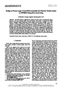
The problem of trajectory tracking for mobile robots has been an attractive issue in the robotic field in recent years. Implementation of classical control methods for this category of robots are usually complicated and time consuming, especially in the case of high mobility robots. Our purpose is to control a certain high mobility rover for rescue operations that has a complex kinematical model. In recent years, expert systems, like fuzzy logic and neural networks have been used and developed for this purpose. The design and selection of linguistic variables and rules of fuzzy controller require expert knowledge of the under control system. This knowledge is usually obtained by trial-and-error or by consulting and observing a human operator controlling a real system. Minimizing both the distance traveled and travel time increases efficiency, but obtaining the optimal set of fuzzy memberships and rules is not an easy task. One of the main factors in the design of efficient and robust fuzzy logic controllers is the selection of parameters of the membership functions. The existing approaches for choosing the membership functions are based on trial-and-error process, which mostly lack learning and autonomy. One method of removing the uncertainty associated with the selection of these variables is the use of evolutionary algorithms (e.g. GA and DE). In this trajectory tracking application the fitness function evaluates the robot’s path taking into account distance and orientation error from the desired path. II. KINEMATIC MODEL OF THE ROBOT A top view of CEDRA rescue robot (see fig. 1) is shown in figure 2. This mobile robot consists of six wheels. Front and rear ones are steerable and the remaining four wheels are mounted beside the robot. Robot kinematic equations can be seen in the equation 1 through 3.
xc (t + ∆t ) = xc (t ) + V (t ). cos(θ (t )). cos(φc (t )).∆t
yc (t + ∆t ) = yc (t ) + V (t ).cos(θ (t )).sin(φc (t )).∆t
(1) (2)
CIS 1066
2 III. FUZZY LOGIC CONTROLLER DESIGN
φc (t + ∆t ) = φc (t ) +
2V (t ) sin(θ (t )).∆t L
(3)
The general configuration of the fuzzy controller, which is divided into four main parts, is shown in figure 4. The first part is the fuzzifier, which converts crisp values into fuzzy sets. Fuzzy sets enter the inference engine as inputs. Fuzzy decisions will be made upon the fuzzy rule base and the results will pass through a defuzzifier stage. Defuzzification is the inverse process of fuzzification. Fuzzy Rule Base Fuzzifier
Defuzzifier Fuzzy Inference Engine
Fig. 4 – The General Structure of Fuzzy Controller Fig. 1 – CEDRA Rescue Robot
Each fuzzy set consists of a number of membership functions to describe the heuristic variables in a mathematical manner. All of the membership functions used in input and output sets are in the form of trapezoid function formulated as in equation (4) [5].
x ∈ (∞, a ] 0, x −a , x ∈ [ a, b) b − a x ∈ [b, c) µ A ( x; a, b, c, d ) = 1, d − x , x ∈ [c , d ) d −c 0, x ∈ [d , ∞) Fig. 2 – Kinematic Model of the Robot
Fig. 3 – Robot and Path Curve Interaction
(4)
A. Fuzzy Input Sets In a Fuzzy Logic controller, the input to the controller (curvature, position error, and orientation error) is converted into a series of fuzzy sets. The number and exact shape of these fuzzy sets critically determine the performance of the controller. These fuzzy sets describe qualitative situations in which the output of the controller is qualitatively different. In other words, whenever the desired behavior (e.g., change from going straight to turning left or change from fast to medium speed) of the controller changes in an input situation, a fuzzy set is created to represent this case. Curvature consists of three fuzzy sets; Left Curvature, Straight and Right Curvature. The fuzzification of the positional error includes five sets; NegHighDist (NHD), NegLowDist (NLD), ZeroDist (ZD), PosLowDist (PLD) and PosHighDist (PHD). It is desirable that the robot being on the line (ZeroDist). Assume that the robot is off the path, then the desired behavior is to turn either right/left towards the path, drive straight towards the path, and then turn left/right to straighten out. Therefore, we require two extra sets on each
CIS 1066
3
side of the path. Similar reasoning leads to the design of the fuzzy sets for the orientation error. A total of five sets have been used to describe different cases; NegHighAngle (NHA), NegLowAngle (NLA), ZeroAngle (ZA), PosLowAngle (PLA) and PosHighAngle (PHA). B. Fuzzy Output Sets There are two outputs from fuzzy controller to robot: (a) speed and (b) steering angle. There are four membership functions for describing the speed heuristic variable: Zero, Slow, Medium & Fast. Steering Angle is determined using five membership functions; SharpLeft (SL), LowLeft (LL), Stright (ST), LowRight (LR) and SharpRight (SR). A crisp output value is then computed from this fuzzy set. This step is called defuzzification. In this research, we used the wellknown centroid defuzzification method, which uses the center of area as the crisp output value. C. Fuzzy Rule Base Given these fuzzy input sets, a fuzzy controller uses a set of fuzzy rules to specify the desired control behavior. After the design of the fuzzy input and output sets, the design of the fuzzy rules is straight forward. There are a total of 5*5*3=75 possible different input configurations. For each of these input configurations, a rule was specified to indicate the desired speed and directional settings. Examples of fuzzy rules appear in Table 1. TABLE 1 FUZZY RULE EXAMPLES
No.
Input
Output
Curvature
d
1
StraightLine
ZD
2
StraightLine
ZD
∆φ
V
Θ
ZA
Fast
ST
PLA
Med
LL
3
StraightLine
ZD
PHA
Slow
SL
4
LeftCircle
NHD
NHA
Slow
SR
5
LeftCircle
NLD
NHA
Slow
SR
6
LeftCircle
NHD
ZA
Slow
ST
7
LeftCircle
PHD
NHA
Slow
LR
8
RightCircle
PHD
ZA
Slow
ST
9
RightCircle
PHD
PLA
Zero
LR
10
RightCircle
PHD
PHA
Zero
SR
IV. EVOLUTIONARY ALGORITHMS A. Genetic Algorithm (GA) Algorithms for function optimization are generally limited to convex regular functions. However, many functions are multi-model, discontinuous, and non-differentiable. Genetic algorithms (GAs) are a class of stochastic search techniques, loosely based on ideas from biological evolution, which have
been used successfully for a great variety of different problems [6]-[8]. The GA searches for an optimal solution from a population of candidate solutions according to an objective function, which is used to establish the fitness of each candidate as a solution. The governing process in the search is the application of appropriate breeding operators to candidate solutions in a given generation to form the candidates for the next generation. These operators are designed to preserve the most successful aspects of candidate fitness until the best possible solution is attained. At each generation, a new set of approximations is created by the process of selecting individuals according to their level of fitness in the problem domain and breeding them together using operators borrowed from natural genetics. This process leads to the evolution of populations of individuals that are better suited to their environment than the individuals that they were created from, just as in natural adaptation. Individuals or current approximation, are encoded as strings, chromosomes, composed with an alphabet, so that the genotypes (chromosome values) are uniquely mapped onto the decision variable (phenotypic) domain. The following steps show the structure and operation of a simple genetic algorithm: 1- Generate strings of random bits from permissible range of variables and place them in free locations in the current population. 2- For each individual in the current population test the objective function then optimize and find the fittest individual and store it. 3- Select first parent via the weighted roulette wheel method. Reproduction, mutation and crossover are three basic operations in evolution. In reproduction parents are carried unaltered into the next generation. Information is exchanged around a randomly generated bit position through crossover, while in mutation randomly generated bit position is altered to a new value. For each function, the user must define a probability that indicates the effect of that function in the evolution. In each section a random number is needed for use in the algorithm. The evolution is based on the statistical nature of these numbers and functions. 4- Steps 2 and 3 must be repeated till the final criterion is satisfied. The final population determines the results of the optimizing problem [9]. B. Differential Evolution (DE) Differential Evolution [3] is an improved version of Genetic Algorithm [10] for faster optimization. The main difference between DE and its antecedent, GA, is using real coding instead of binary coding to represent problem parameters. We can list many advantages for DE including simple structure, ease of use, low number of control parameters and speed. The simple adaptive scheme used by DE ensures that these mutation increments are automatically scaled to the correct magnitude. DE uses non-uniform
CIS 1066
4
crossover in which the child inherit the parameter values from the parent vectors in unequal properties. In reproduction, the child vector competes against one of its parents in order to be selected. DE is a parallel direct search method with NP parameter vectors in the form of xi,G (i=0,1,…,NP-1) for each generation (G) population. Number of population (NP) is fixed during the optimization process. If there is no assumption for initialization or knowledge about the system, the initial population may be chosen randomly with a normal probability distribution. DE utilizes a new scheme for generating trial parameter vectors. In DE, new parameter vectors are generated by adding the difference vector between two population members to a third member with an adjustable weight factor. Next, a comparison will be done between the newly generated vector and a predetermined vector and the one with the lower objective function value will survive. One of the most promising versions of DE algorithm generates a trial vector v for each vector xi,G (i=0,1,…,NP-1) by the following relation
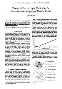
The existing iterative approaches for choosing the membership functions are basically a manual trial-and-error process and lack learning capability or autonomy. Therefore, the more efficient and systematic evolutionary optimization algorithm which act on the survival-of-the-fittest has been applied to FLC design for searching the poorly understood, irregular and complex membership function space with improved performance. From the point of view of evolutionary search, membership functions can be seen as functions, the parameters of which are necessary to achieve optimization in general terms and are independent of sensory application. Figure (5) shows a sample of a parametric membership function with eight parameter; a1 ,…., a8. The goal is to achieve to minimum distance summation in path tracking. Since some rules may be uncertain weight of the rules are optimized too. The range of membership function parameters are determined based on robot and path dimensions. The objective function in mathematical formulation as applied to this work is: imax
v = xr1,G + F. (xr2,G - xr3 ,G)
(5)
obfun = ∑ Distance(i )
(7)
i =1
where integers r1, r2, and r3 are mutually different and belong to the interval of [0,NP-1]. F is a positive, real and constant factor which controls the magnitude of differential variation and is called the scaling factor [3]. There are lots of alternatives for the above mentioned trial vector generation scheme. The second version works in the same way as the first one but the vector v is calculated according to equation (6). v = xr1,G +λ.( xbest,G - xri ,G)+ F. (xr2,G - xr3 ,G)
(6)
where λ is an additional control variable and xbest,G is the best parameter vector for each generation G. The second scheme can be useful for non-critical objective functions [3]. Then in every generation, in order to increase the diversity of the parameter vector, each primary array vector is going through a crossover phase to produce a trial vector. Thus the trial vector is the child of two parents, a noisy random vector and the target vector against which it must compete. The nonuniform crossover is used with a crossover constant CR, in the range 0 =< CR Dmax or x > xmax or x < xmin
(9)
Fig. 5 – Sample of Parametric Membership Function
Optimization process has been fulfilled using the two evolutionary algorithms mentioned earlier; GA and DE. We have developed a modified version of DE which preserves the initial variable intervals in order to eliminate the unacceptable solution space. Algorithm parameters and their performance comparison have been shown in Table 2. As can be seen, the number of population and generations is set to be equal in both methods and achieved error summation and mean have been compared.
CIS 1066
5
TABLE 2 ALGORITHMS PARAMETERS AND PERFORMANCE COMPARISON Parameter Name
GA
DE
NP (Number of Populations)
100
100
No. of Variables
20
20
Maximum Generation F (Scaling Factor)
200
200
-
0.6
-
0.7
CR (Crossover Probability) Ggap (Generation Gap)
0.9
-
Lind (Length of Individual Vars. ) Crossover Rate
10
-
0.9
-
Mutation Rate
0.07
-
Error Summation
19879
19377
No. of Sampling
399
411
49.9 (mm)
47.2 (mm)
Average Error
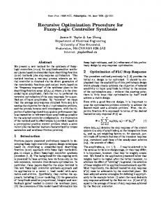
The mentioned errors correspond to the tracking of an assumed test path with a highly complicated shape and sharp edges. Results have demonstrated that both algorithms performances are mostly the same, although error summation and mean achieved by DE is slightly lower than its competitor; GA. As can be seen DE has gained an average error 5.4% lower than GA. Another advantage of DE is its lower number of control parameters which makes it easier to use. Simulations are presented using a complicated path including several break points to show the controller’s performance. At any instant, the position and orientation of the robot are assumed to be determined by an accelerometer and tilt sensor. Data sampling time of controller is set to 0.5 s. Although the sampling time is relatively large, the tracking controller has responded in an acceptable way. Figure (6) shows the response of an initial fuzzy logic controller. Figures (7) and (8) depict the performance of an optimized fuzzy logic controller using GA and DE respectively. As can be seen, the deviation from the desired path has been extremely reduced after optimization independently of algorithm type. We can observe similar results of the two utilized techniques in practice as well.
Fig. 6 – Path Tracking Before Optimization
Fig. 7 – Path Tracking After Optimization by GA
Fig. 8 – Path Tracking After Optimization by DE
CIS 1066
6
VI. CONCLUSION In this paper, a fuzzy logic controller has been developed for path tracking of a rescue robot. In order to tune the membership functions, (to achieve minimum deviation from the desired path) we have used two evolutionary methods; Genetic Algorithm and Differential Evolution. The improved performance of the controller relative to the original has been shown via tracking simulation over a complicated path. According to the results, performance of the optimized controller is more acceptable than the initial controller. A comparison between the two mentioned algorithms has also been addressed and they were found to have similar results except slightly lower error and having less control parameters for the DE method.
REFERENCES [1]
C. A. Floudas, Nonlinear and mixed-integer optimization. Oxford University Press, New York, 1995. [2] D. Dasgupta, and Z. Michalewicz, Evolutionary Algorithms in Engineering Applications, Springer, Germany, 1997, pp. 3 - 23. [3] K. Price, and R. Storn, "Differential evolution – a simple evolution strategy for fast optimization," Dr. Dobb’s Journal, vol. 2, no. 4, 1997, pp. 18 – 24 and 78. [4] B.V. Babu and R. Angira, “Optimization of non-linear chemical processes using evolutionary algorithm,” Proceedings of International Symposium & 55th Annual Session of IIChE (CHEMCON-2002), OU, Hyderabad, December 19-22, 2002. [5] L. X. Wang, A Course in Fuzzy Systems and Control. Prentice-Hall Int., Englewood Cliffs, NJ, 1997, p. 129. [6] K. A. De Jong, "Analysis of the behavior of a class of genetic adaptive systems," Ph.D. thesis, The University of Michigan, Ann Arbor, MI. [7] D. E. Goldberg and M. P. Samtani, "Engineering optimization via genetic algorithm," Ninth Conference on Electronic Computations, 1986, pp. 471-482. [8] J. J. Grefenstette and J. M. Fitzpatrick, "Genetic search with approximate function evaluation," International Conference on Genetic Algorithms and Their Applications, 1985, pp. 112-120. [9] D.E. Goldberg, Genetic Algorithms in Search, Optimization and Machine Learning, Addison-Wesley Publishing Co., Boston, MA, 1989. [10] C. N. Kim and L. Yun, “Design of sophisticated fuzzy logic controllers using genetic algorithms,” Proc. 3rd IEEE Int. Conf. On Fuzzy Systems, Orlando, FL, vol.3, 1994, pp. 1708-1712.