Gawthrop, P.J. and Wang, L. (2005) Data compression for estimation of the physical parameters of stable and unstable linear systems. Automatica 41(8):1313-1321.
http://eprints.gla.ac.uk/archive/00001966/
Glasgow ePrints Service http://eprints.gla.ac.uk
Data Compression for Estimation of the Physical Parameters of Stable and Unstable Linear Systems Peter J Gawthrop a,1 Liuping Wang b a Centre
for Systems and Control and Department of Mechanical Engineering, University of Glasgow, GLASGOW. G12 8QQ Scotland.
[email protected]
b Discipline
of Electrical Energy and Control Systems, School of Electrical and Computer Engineering, RMIT University, Melbourne, Victoria 3000, Australia
Abstract A two-stage method for the identification of physical system parameters from experimental data is presented. The first stage compresses the data as an empirical model which encapsulates the data content at frequencies of interest. The second stage then uses data extracted from the empirical model of the first stage within a non-linear estimation scheme to estimate the unknown physical parameters. Furthermore, the paper proposes use of exponential data weighting in the identification of partially unknown, unstable systems so that they can be treated in the same framework as stable systems. Experimental data are used to demonstrate the efficacy of the proposed approach. Key words: Parameter estimation; partially known systems; basis function.
1
Introduction
Many engineering systems of interest to the control engineer are partially known in the sense that the system structure, together with some system parameters are known, but some system parameters are unknown. This gives rise to a problem of parameter estimation when values for the unknown parameters are to be determined from experimental data comprising measurements of system inputs and outputs. There is a considerable literature in the area (An, Atkeson, and Hollerbach, 1988; Canudas de Wit, 1988; Dasgupta, Anderson, and Kaye, 1986; Gawthrop, Jones, and MacKenzie, 1992; Gawthrop, 2000a,b; Nagy and Ljung, 1991). Although, in special cases, such identification may be linear-in-the parameters (An et al., 1988) or polynomial-in-the parameters (Gawthrop et al., 1992), in general the problem is nonlinearin-the parameters. This means that, in general, the resultant optimisation problem is not quadratic or polynomial, and may even be non-convex. In such cases, the optimisation task is eased by knowing (rather than deducing numerically) the derivative of the error function with respect to the unknown system parameters. The generation of such sensitivity information is aided by the symbolic methods for nonlinear systems modelling, analysis and optimisation which are currently strong research areas (Munro, 1999) driven by the 1
Corresponding author
Preprint submitted to Automatica
ready availability of symbolic computational tools. In particular, the bond graph approach (Gawthrop and Smith, 1996; Karnopp, Margolis, and Rosenberg, 1990; Ljung and Glad, 1994) has been used to generate models both applicable to control design (Gawthrop, 1995; Gawthrop and Ronco, 2000) and partially-known system identification (Gawthrop, 2000a, 2003; Nagy and Ljung, 1991). Bond graph models are used in all the examples of this paper, but are not discussed further here. Data acquisition systems typically yield large amounts of discrete-time data. On the other hand, the aforementioned partially known systems are usually best expressed in continuous-time differential equation form and, even with these sensitivity function enhancements, use of the raw data may lead to unacceptable computational times. Thus, although it is, in principle, possible to use algorithms for partially-known system identification directly on the raw data, it is not practically useful. In addition, the raw data may contain complex system disturbance information which may require a sophisticated optimisation algorithm to achieve desirable results. In this paper, the authors propose a two-stage identification procedure to extract physical parameters from discrete-time data pertaining to partially known systems. The first stage (which we call data compression) analyses the raw data to obtain a parameter vector θ describing an empirical model obtained from the data. The second stage uses this empiri-
24 February 2005
cal model (parameterised by θ) to generate continuous-time data suitable for identifying physical parameters. Because the first stage is essentially a linear-in the parameter problem, not only can large amounts of data be processed rapidly, but also established system identification tools can be used to obtain data-quality models (Ljung, 1999). Because the second stage uses a relatively short length of relatively noise free data, the iteration time and convergence properties are much improved compared to using the raw data directly. The continuous time step response is used as the empirical model as it has a transparent representation in terms of gain, time delay and time constant and thus it is widely accepted by engineers and practitioners. Other forms of empirical model are also possible within this context. The basic idea of a two-stage method is not new, see for example, Ljung (1999, Section 10.4) and Wang, Gawthrop, Chessari, Podsiadly, and Giles (2004); our method is new insofar as it uses the FSF approach for the first stage and a physical model-based approach for the second.
sampling-rate independent values. This latter approach is discussed in Section 2.1 and extended to unstable systems in Section 2.2.
2.1
Stable systems
1
1
0.8 0.8
0.6 0.4
0.6
Im
|H|
0.2
0.4
0 −0.2 −0.4
0.2
−0.6 −0.8
0
In order for the same framework to be applicable to unstable systems, this paper proposes the use of exponential data weighting in the data compression procedure. This exponential weighting converts an unstable system into a stable system with the same unknown parameters to which the two-stage approach is applicable.
0
1
2
3
4 5 6 omega
7
8
−1 −1
9 10
(a) Frequency responses
−0.5
0 Re
0.5
1
(b) Pole locations
0.25 0.2 0.15 0.1 0.05 Im h
The motivation for this work is to generate models suitable for model-based predictive control (Mayne et al, 2000; Rawlings, 2000), in particular models suitable for continuous time methods, such as those of Wang (2001) and Gawthrop and Ronco (2000, 2002).
0 −0.05 −0.1 −0.15 −0.2 −0.25 0
2
1
2
3
4
5
t
The outline of the paper is as follows. Section 2 considers the frequency sampling filter approach to data compression and extends the procedure to cope with unstable systems. Section 3 considers physical parameter estimation and section 4 considers frequency-domain approaches. Section 5 gives illustrative experimental results using data obtained from both electrical and electro-mechanical systems. Section 6 concludes the paper.
(c) Time responses Fig. 1. Frequency-sampling filters
The book by Wang and Cluett (2000) gives a comprehensive discussion of the frequency-sampled filter approach (including its relation to the discrete Fourier transform); this section provides a brief discussion of the material required for this paper. We consider linear time-invariant continuoustime systems with output y(t) and input u(t) uniformly sampled with time interval ∆ to give input and output sequences yi = y(i∆) and ui = u(i∆). In the time-domain, the input and output sequences are related by yi = gi ∗ ui where gi is the discrete-time system impulse response and ∗ is the convolu¯ U(z) ¯ tion operator. In the z-transform domain, Y¯ (z) = G(z) where Y¯ and U¯ are the z-transforms of yi and ui respectively and G¯ the corresponding transfer function. In this section, it is assumed that the system is stable and can be associated with a settling time T = N∆; the time after which the system impulse response is sufficiently small: |gi | < ε ∀i > N.
Data compression
The first stage of the two-stage process is data compression: encapsulating the important features of the measured data into a few parameters within an empirical system model. There are many possible empirical models available including ARX (Ljung, 1999) and general basis-function approaches (Ninness and Gustafsson, 1997; Wahlberg, 1991; Wang and Cluett, 2000). In a fast-sampling environment, it is known that discrete-time ARX models encounter numeri˚ om, Hagander, and Sternby, 1980) cal ill-conditioning (Astr¨ as the sampling rate increases; and the problem is worse for unstable systems. On the contrary, the frequency-sampling filter (FSF) approach of Bitmead and Anderson (1981); Wang and Cluett (1997, 2000), lies between the continuous and discrete-time domains and the coefficients converge to
The frequency-sampling filter FSF approach approximates
2
¯ the transfer function G(z) as: n−1 2
∑
G¯ f s f (z) =
θk H¯ k (z)
usual time-domain filtering operation. Equation (4) is in the conventional linear-least squares form and so the parameter estimate θˆ may be chosen to minimise a performance index of the form
(1)
M
ˆ = ∑ |ei |2 J(M, θ)
k=− n−1 2
1 1 − z−N H¯ k (z) = N 1 − e jΩk z−1
(2)
where ei = yi − yˆi and yˆi is given by (6) with θ replaced by ´T ³ ˆ Defining YM = y0 y1 . . . yM , φi = fi ∗ ui and ΦM = θ. ´T ³ then the Least Squares estimate is φ0 φ1 . . . φM
where n is odd and the frequency sample interval Ω = 2π T H¯ k (z) is the kth frequency sampling filter (FSF) and θk the corresponding (complex) parameter. The name arises because the kth FSF has a frequency response with a peak at ω = kΩ. Figure 1(a) shows the superimposed frequency responses of H¯ k (z) for 0 ≤ k ≤ 4 when T = 5 implying Ω = 1.26 for a frequency range 0 ≤ ω ≤ 10. The symbol “x” marks the frequency samples which coincide with the peaks of the FSFs. The kth filter of (2) has the discrete-time impulse response h¯ k (i) 1 h¯ k (i) = e jΩki i < N N
θˆ = (Φ∗M ΦM )−1 Φ∗MYM
As discussed by Wang and Cluett (1997, 2000), choosing ¯ n = N gives an exact match G¯ f s f (z) = G(z). Choosing n < N ¯ gives an approximate match G¯ f s f (z) ≈ G(z) for a frequency range 0 ≤ ω ≤ NΩ. This situation is summarised in Figure 1(b) which shows N = 50 potential FSF poles (marked by “+”) equispaced around the unit circle and the n = 9 actual FSF poles clustered around z = 1 on the unit circle. Particularly in the context of fast (with respect to system time constants) sampling, a good approximation can be obtained with n