GENETIC ALGORITHMS APPLIED FOR PATTERN GENERATION FOR DOWNHOLE DYNAMOMETER CARDS L. Schnitman1; B.C.Brandao1; H.Lepikson1; J.A.M. Felippe de Souza2 ; J.F.S.Correa3 1
2
Universidade Federal da Bahia- Brazil Universidade da Beira Interior, Covilhã – Portugal 3 Petrobras – UN-BA - Brazill
[email protected] ;
[email protected] ;
[email protected]; ;
[email protected];
[email protected]
Abstract: Rod-pumping is a largely used technique for oil extraction. Pumping conditions and malfunctions may be monitored through downhole dynamometer cards (DC). DCs are a load vs. position plots of the pump. Its monitoring is important to sustain acceptable productivity levels. An automated system for DC shape classification is desired for quicker response avoiding production disturbances. PETROBRAS has such a system that relies on a set of pattern tables, which are used to match the DCs. However, the problem of pattern identification and generation still remains. This article proposes a new method for patterns generations based on genetic algorithms (GA), so that DCs can be better classified by the used method. Copyright @Controlo 2004. Key-Words: recognition, genetic algorithms, pattern generation, rod-pumping 2. 1.
DOWNHOLE DYNAMOMETER CARD
INTRODUCTION
Monitoring oil wells production is a hard task which requires several details in order to sustain acceptable productivity levels. Rod-pumping is one of the most used techniques for oil extraction as well as DCs are one of the main tool for rod-pumping well production analysis. PETROBRAS has such a system that relies on a table of patterns and uses a specific method to match the DCs. The used method operates satisfactorily, although with a reduced number of shape types classifiable. It requires one pattern for each classifiable DC shape type. When tested against the actual table, the pattern that has the closest match is choosed to indicate the DCs shape type. This article describes a new approach for pattern generation based on genetic algorithms so that previous results can be improved in terms of numbers of patterns to be classified and their respective accuracy. Section 2 describes the set of theoretical DCs which are desired to be recognized. In section 3, the actual used method is described. The concepts of GA application are introduced in section 4 and section 5 presents its application. Section 6 presents some numerical results. Conclusions are detailed in section 7.
DCs shapes indicate certain pumping characteristics or states. Those cards are acquired periodically from the wells and stored in a database. They consist of a collection of bidimensional points, where the X axis represents the displacement of the pump, and the Y axis the load. The plotting begins at the lower left corner of the card, with the pump unloaded at the bottom of the well, and goes on circle clockwise until the pump returns to the initial position. A slightly more detailed description can be found at [7]. An example of real DC data is shown in Figure 1.
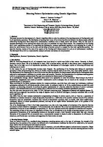
Figure 1: DC real data There are many theoretical shapes described in the literature [1], from which 8, as shown in Figure 2, are the main interest of this article. All of them describe clearly a predominant effect and they were selected by PETROBRAS expert engineer [1].
1-Normal, unanchored tubing
Many combinations of conditions and malfunctions are possible. Of course, its classification becomes more difficult when more complex operating conditions occurs. However, they can not be generalized, therefore are not covered in this article. 3.
ACTUAL RECOGNITION METHOD
The objective of the recognition system is to classify a certain DC data as one of the shape types previously chosen. For that purpose pattern table is needed. 2-Severe fluid pound
3-Severe gas interference
4-Rod stuck by sand
5-Leaking standing valve
For each shape type there is one pattern that is compared with the DC data in order to generate a confidence degree. During operation, the DC data is tested against each one of the patterns available so that the highest confidence identifies the closer shape type. The DC data may show variations in scale and offset. Thus, the first step is then to normalize the data. It is important to note that data comes with a high degree of redundancy. In order to improve time delay, memory use and storage efficiency, data are compressed by known method [2]. The main idea of the proposed method is based on variation of direction beyond a specified threshold so that the original plot can be approximately reconstructed by interpolation methods [3]. Compressed data are called as representative plots (RP) from now on and represents a set of (X,Y) pairs that represents the main DC data. Figure 1 presents a didactic example of DC card while Figure 4 present its reconstruction by the RP shown as red circles when a sensibility of 15o is used for the angle variation detection. A circle as a didactic example of DC card 700 650 600
6-Leaking traveling valve
550 500 450 400
7-Pump tapping at the top
350 300 300
350
400
450
500
550
600
650
700
Figure 3: Didactic example of DC card
8-Pump tapping at the bottom Figure 2: DC patterns
Remark 1: It is important to note that this is the method which is used by PETROBRAS in real cases so that faults or benefits of the method do not compose the contents of this paper. On the other hand, satisfactory results are described by expert operators. Also, note that its application requires a known pattern table such that the problem of pattern generation still remains.
Reconstruction based on RP 700 650 600 550 500 450
4.
400 350 300 300
350
400
450
500
550
600
650
700
Figure 4: Reconstruction by the RP (red circles) Compressed data are then to be tested against the recognition patterns. The patterns consist of a small number of bidimensional points (X,Y) and their respective variance (V) and relevance (R). The variance V of a point is used to account for the divergence between the position of that pattern’s point position and the closest RP. The relevance R weights the patterns points so that points which belongs to regions of the graph that are more significant for the shape type have higher weight, and vice-versa. Consider Pi a specific point (X,Y) of an acquired DC. The test procedure is as follows: a) Choose a new point Pi from the DC b) Find the point from the RP, RPj, that has the shortest euclidean distance Di from Pi. Min (Di2 = (RPjx – Pix)2 + (RPjy – Piy)2) c) Compute a partial confidence ci for that point according to the distance Di using: ci = -0,5x+1 where x =
Di Vi
d) After performing a, b and c once for every point in RP, compute the resulting confidence C using the partial confidences and the relevance Ri of each Pi, Ri:
∑c R C= ∑R i
i
i
i
i
e)
The highest resulting confidence indicates which class the DC belongs to.
The whole procedure can be summarized as: - Normalize data - Compress the data – extract RPs - Test against each pattern: compute resulting confidence for each one of them. - Choose the shape type whose pattern has given the highest confidence.
GENETIC ALGORITHM
An automatic method for pattern generation is strongly recommended to enhance the actual method. Genetic algorithms (GA) are a search algorithm with adequate performance, especially used when formal approach is hard to be implemented or has no efficient results. They are inspired in the Darwin’s theory of evolution. An accessible introduction to GA can be found at [4][5][6]. Given a search space, an initial population (set of possible solutions) and a fitness function used to compute the solution performance, and adequate GA may search for regions of maximum or minimum, which is supposed to hold adequate better performance with respect to the fitness function. The GA search method is based on the evaluation of the population. It happens through crossover and mutation by a certain number of generations. For each generation each chromosome (individual) of the population has its adaptation degree performed by the fitness function. Higher degrees associate higher probabilities of combining, and therefore, maintain their characteristics in future generations which has higher surviving probability. This paper uses the GA parameters: a) Population size: Number of chromosomes, or individual solutions. Big values slow down significantly the evolution; small values usually lead to premature convergence, situation where the algorithms get stuck at a local extreme with probable sub-optimal solutions. b) Probability of crossover: Associated to the probability of recombination of the chromosomes. This value is usually set high, lower values slow down the convergence. c) Probability of mutation: Associated to how often the chromosome will have his characteristics randomly altered. This value is usually kept low. Higher values may lead to a random search. d) Population overlapping: Associated to a number of individuals of the old generation that should be maintained at the new generation. Keep the best chromosomes is a usual procedure for evolutionary purposes.
It is called as elitism and guarantees that the next generation contains at least the best solution of the last one. 5.
PATTERN GENERATION PROPOSED METHOD
The problem of the pattern recognition used method is how to generate N patterns to respective N shape types that the system should recognize through an automated way. The objective is to be able to correctly classify DC’s types. In order to evaluate the proposed algorithm performance, a known data base is used. It has 6.428 plot samples from different wells and different shape types and contains the normalized acquired data of load vs. position plots, the extracted RP and also the respective DC type based on previous classification. Each chromosome of the GA is set to be a real number array of fixed length. This array is divided in groups of four numbers, consisting of the Cartesian coordinates (X,Y), the relevance (R) and the variance (V). A set of 10 groups represents a pattern proposition. One concludes that evolving all the patterns at the same time would be less efficient, since it would require a larger population and the proposed algorithm convergence may be delayed. Thus, each pattern has a specific population and higher number of individuals is used. The proposed approach is to separately treat each pattern. However, the evolution is done at the same time in such way that the individual result of a specific pattern performance may be used and compared with the other ones. The algorithm begins by testing the population (patterns propositions) against the whole database. It results a confidence table TC, which contains the confidence values for every sample and every pattern. Each individual confidence value is obtained as explained in section 3.
evaluated as the difference between the chromosome match ratio (1-error ratio) and the highest error ratio from the other N-1 patterns that are not being evolved at the given time. At each generation, every chromosome of the population is tested against every sample at the database. For each chromosome a new report table is generated. For this, the resulting confidences for each sample are checked against the stored values from the other N-1 patterns in TC. Therefore a new report table is generated, with corresponding match and error ratios of each pattern and the fitness value of each chromosome can be evaluated. The system is left evolving until: a) There is another pattern that has a higher error ratio. In that case, the system is set to evolve this pattern. That is, the TC is updated with the confidence values from the best chromosome that represents the pattern that was being evolved previously. Therefore the pattern’s column in TC is replaced with the new values. A new population is created and the new pattern inserted in it, and let, as already described, evolving. b) There have been many generations since the last time a better chromosome were found. In that case, the GA seems to be stuck, and the system is set to evolve the pattern that has incorrectly detected more DC’s of the pattern that was being evolved. A procedure similar to “a” is used. For an example see table 2. Five samples from type 1 were incorrectly recognized as type 6; in that case, if the system were stuck trying to evolve the pattern 1, the pattern 6 would be set to evolve instead. c) The system is not changing again but “b” has already been attempted. In that case, a random pattern is chosen to be evolved. 6.
RESULTS
The highest confidence value indicates from which type the sample is recognized to be into. Since the actual type of the sample is known from the database, it is possible to evaluate right and wrong recognition. A report table is then generated describing the number of DC’s that are rightly recognized and the number that are not (see table 2 for an example). This way the recognition error ratio is known for each pattern.
Previous values for the GA parameters are used as: - 80% of crossover probability - 0.5% mutation probability - population size of 30 to 50 chromosomes - population overlap of 2
The algorithm starts by picking the pattern with the highest error ratio and try to evolve a better one through the GA. A new population is created and the chosen pattern inserted in it as a chromosome. The fitness value that is actually used by the GA is
Erro! A origem da referência não foi encontrada. presents the results when the proposed algorithm is used and previous parameters are sets. It summarizes the obtained results when compared with expert knowledge stored in the Data Base. Each column
In Table 1, pattern types are associated to Figure 2 description while “Not found” means that the pattern can not be found in the used data base.
It means that considering a table of expert knowledge classification, the algorithm is able do automatically generate a table of patterns which summarizes the expert knowledge and may be used for automatic classification of DC.
presents the classification of the respective DC type. For instance, one has 1937 classifications of normal DCs (type “1”, see Table 1) which are classified as pattern “1” (1930 of them), pattern “2” (2 of them) and pattern “6” (5 of them). It means that only 7 errors happened.
REFERENCES [1] Corrêa, J. F. “CartaPad – Cartas Dinamométricas Padrões” Apresentado no II Seminário de Engenharia de Poço, Rio de Janeiro, 1998.
Pattern Data Base Type Registers “1” 1.937 “2” 4.342 “3” 17 “4” Not found “5” Not found “6” 84 “7” 48 “8” Not found TOTAL 6.428 Table 1: Expert knowledge based pre-classified Data Base
7.
[2] Regattieri, M., Andrade Neto, M., Rocha, A. F. “Results of Data Compression for Plane Curves Using Neural Networks” Proceedings of IEEE Neural Nets Congress, Orlando, v. , p. 1691-1694, 1994. [3] Regattieri, M., Zuben, F. J. V., Rocha, A. F. “Neurofuzzy Interpolation: II – Reducing Complexity of Description” 2nd International Conference on Neural Networks IEEE San Francisco, p. 1835-1840, 1993. [4] Forrest, S. “Genetic Algoritms” ACM Computing Surveys, Vol. 28, No. 1, 1996.
CONCLUSIONS
A significant computational effort is required for pattern generation. On the other hand, it should not be considered for practical solutions. The presented algorithm is not proposed to be an on-line training method. Thus, a single pattern table is required for practical implementation.
[5] Obitko, M. “Introduction to Algorithms” http://cs.felk.cvut.cz/~xobitko/ga
[6] Wall, M. “GAlib: A C++ Library of Genetic Algorithm Components” ver. 2.4 Doc. rev. B, 1996.
The obtained result shows that the algorithm performance is adequate and patterns are generated in such a way that the pattern recognition method enhances its performance while it tries to reproduce the human expert knowledge.
Recognized Type 1 2 3 4 5 6 7 8 Total Error %
1
2
1930 2
4339
Genetic 1998,
[7] “TechNote: Pump Card Shapes”, http://www. echometer.com/support/technotes/pumpcards.html
Database Sample (DC Type) 3 4 5
6
7
8
17 1 5
1 2
1 84 48
1937 7 0,36
4342 3 0,07
17 0 0,00
1 0 0,00
1 0 0,00
84 0 0,00
48 0 0,00
1 1 0 0,00
Table 2: Obtained results Remark 2: Since some types of DC are not found in the Data Base, a single example is artificially generated to represents each one of them.