Good modelling practice in applying computational fluid dynamics for ...

Uncorrected Proof 1

© IWA Publishing 2015 Water Science & Technology

|

in press

|

2015

Good modelling practice in applying computational fluid dynamics for WWTP modelling Edward Wicklein, Damien J. Batstone, Joel Ducoste, Julien Laurent, Alonso Griborio, Jim Wicks, Stephen Saunders, Randal Samstag, Olivier Potier and Ingmar Nopens

ABSTRACT Computational fluid dynamics (CFD) modelling in the wastewater treatment (WWT) field is continuing to grow and be used to solve increasingly complex problems. However, the future of CFD models and their value to the wastewater field are a function of their proper application and knowledge of their limits. As has been established for other types of wastewater modelling (i.e. biokinetic models), it is timely to define a good modelling practice (GMP) for wastewater CFD applications. An International Water Association (IWA) working group has been formed to investigate a variety of issues and challenges related to CFD modelling in water and WWT. This paper summarizes the recommendations on GMP of the IWA working group on CFD. This paper provides an overview of GMP and, though it is written for the wastewater application, it is based on general CFD procedures. A companion paper forthcoming to provide specific details on modelling of individual wastewater components forms the next step of the working group. Key words

| CFD, GMP, protocol, wastewater treatment

Edward Wicklein (corresponding author) Carollo Engineers, 1218 Third Ave, Suite 1600, Seattle, WA, USA E-mail: [email protected] Damien J. Batstone Advanced Water Management Centre, University of Queensland, Level 4, Gehrmann Laboratories Building (60), Brisbane, QLD 4072, Australia Joel Ducoste Department of Civil, Construction, and Environmental Engineering, North Carolina State University, Campus Box 7908, Raleigh, NC 27695-7908, USA Julien Laurent ICube, Université de Strasbourg, CNRS (UMR 7357), ENGEES, 2 rue Boussingault, 67000 Strasbourg, France Alonso Griborio Hazen and Sawyer, 4000 Hollywood Boulevard, Suite 750N, Hollywood, FL 33021, USA Jim Wicks The Fluid Group, The Magdalen Centre, Robert Robinson Avenue, The Oxford Science Park, Oxford, OX4 4GA, UK Stephen Saunders Ibis Group, 101 NW Seminary Ave, Micanopy, FL 32667, USA Randal Samstag Civil and Sanitary Engineer, PO Box 10129, Bainbridge Island, WA 98110, USA Olivier Potier Laboratoire Réactions et Génie des Procédés, Université de Lorraine CNRS (UMR7274), 1 rue Grandville, 54001 Nancy, France Ingmar Nopens BIOMATH, Department of Mathematical Modelling, Statistics and Bioinformatics, Ghent University, Coupure Links 653, B-9000 Ghent, Belgium

doi: 10.2166/wst.2015.565

Uncorrected Proof 2

E. Wicklein et al.

|

Good modelling practice in applying computational fluid dynamics

Water Science & Technology

|

in press

|

2015

INTRODUCTION Computational fluid dynamics (CFD) models have been extensively and successfully used in a wide range of engineering disciplines including, but not limited to, automotive engineering, chemical engineering, mechanical engineering and aerospace engineering for many decades. In recent years, there has been a steady increase in CFD modelling in the wastewater treatment (WWT) field, both in academia (universities and research institutes) and industry (consultants and manufactures). This growth is due to increased availability of quality CFD models, increasing power and affordability of computing power, and increased importance of drivers for optimization of municipal and industrial WWT unit processes. CFD models are powerful tools that have become increasingly available with commercial packages providing graphical user interfaces to assist with model development, operation, and post processing. However, WWT unit processes involve a complex interaction of fluid, mechanical, biological, and chemical processes. Therefore, despite the improved prospects for application of CFD, these models still require significant expertise and experience to produce good quality and, hence, useful results. A limitation noted by Nopens et al. () is that there are currently few CFD modelling experts within the environmental educational and academic sector. This lack of educational support can lead to software misuse by inexperienced users. Misuse leads to erroneous outcomes, which can result in bad designs or processes that result in suboptimal hydraulic design, contributing to distrust of CFD models in the WWT field. While there are several textbooks available on the general use of CFD modelling, currently there is no textbook or scientific report available that addresses practical applications of CFD specifically for WWT. Based on this lack of available guidelines, the IWA has recently chartered a working group on CFD modelling to address issues of applying CFD to WWT engineering as well as training of CFD engineers. In addition, the relevance of precise details within WWT were historically not as significant when discharge limits were less stringent, energy input was less critical, the facilities were sized for a future conditions.

Figure 1

|

Overview of WWT unit processes commonly modelled using CFD.

In contrast, other industries with a longer history of CFD model use and more stringent fluid flow requirements have established clear guidelines for quality modelling. Key references include Roache (), the 1998 American Institute of Aeronautics and Astronautics Guide to Verification and Validation of CFD Models, and the ERCOFTAC Best Practices Guidelines (Casey & Wintergerste ) for CFD modelling. A typical WWT works activated sludge liquid stream treatment system is illustrated in Figure 1. The hydraulics of many of these components have been modelled using CFD, and there are numerous examples in the literature including pumps (Li et al. ), primary sedimentation (Liu & Garcia ), chemically enhanced primary treatment (McCorquodale et al. ), activated sludge (Le Moullec et al. b), secondary clarifiers (De Clercq ), membrane’s (Brannock et al. ), disinfection systems included UV (Ho et al. ) and chlorine contactors (Khan et al. ), outfalls (Khan et al. 2005), and digesters (Bridgeman ). In addition, the physical, chemical, and biological processes occurring within the fluid are increasingly modelled to better understand the performance of the unit process. Despite this growth, application of CFD has not reached comparable levels to other engineering fields, where it is standard for prototyping and evaluating equipment and assessing factors that would not normally be evaluated by other approaches. Besides the limitations mentioned earlier, the lack of significant use of CFD for the optimal design of WWT unit processes in Figure 1 may be due to the lack of full scale experimental validation of CFD models, leaving CFD models primarily to sort out the impact of design changes on hydraulic performance through relative comparison between different model configurations. General components of good modelling practice (GMP) for any modelling exercise are illustrated in Figure 2 (Hangos & Cameron ). These consist of (1) clearly defining the objective of the modelling task with all project parties involved; (2) collection of data, defining the model configuration (e.g. level of detail of the model, spatial discretization or mesh generation) and simulation settings; (3)

Uncorrected Proof 3

E. Wicklein et al.

|



|

in press

|

2015

needed for the problem. In general, the least amount of computational effort should be used to answer the design or research question being sought from the model results. The modeller must determine if the problem can be defined in two or three dimensional space; if the problem is steady state (boundary conditions and solution are time independent) or dynamic; if the problem is single species, single phase with multiple species, or multiphase; if the problem is Newtonian or non-Newtonian; if there is heat transfer, and if additional transport, momentum transfer or mass transfer equations are needed for solutions of secondary species, phases and reactions. Once the modelling approach is determined, model development begins with defining the problem geometry including the key physical details influencing the flow and process being simulated. In many cases, the modeller has to balance complexity with computational efficiency. As an example, small details that do not significantly influence the bulk flow field and are on the order of, or significantly smaller than the computational mesh size are often neglected. This step is followed by meshing, application of boundary conditions, flow solution, and post processing. Each of these activities has minimum requirements to develop quality results, all of which will be discussed in more detail in the following sections. Figure 2

|

Overview of the different components of a general modelling process.

running the simulations (steady state, dynamic), and (4) post-processing, calibration, and validation. After these steps, either the objective is met or the developed model is ready to be used to explore the answer to the objective with additional methods such as scenario analysis. An important addition prior to the objective is the question of whether a CFD model is required. The question of using CFD is important given the computational load of these models. If the objective can be reached using a simpler model, then that option should be the preferred choice. As a similar interest and need exists for wastewater CFD applications, this paper’s objective is to outline GMP for use of CFD models in WWT. It is noteworthy that these recommendations stem from general CFD application. General GMP protocol for CFD modelling in wastewater treatment The overall CFD modelling approach and process is outlined in Figure 3. After identifying the objective, a system analysis is conducted to determine the level of physics

Approach and key assumptions Several key choices need to be made at the outset of any CFD modelling problem to guide the direction of the modelling process. These choices include (1) spatial dimensionality; two vs. three dimensions; (2) time averaged versus time marching; (3) the number of phases and species; (4) material properties and their interactions when multiple species are present, and (5) if additional transport or transfer models are needed beyond what is already included in the CFD package. In terms of spatial dimensionality, a three-dimensional (3D) problem may not substantially require more user effort to set up as opposed to a two-dimensional (2D) problem. However, it may have a significant impact on computational requirements due to the increased degrees of freedom. Hence, one should check whether the assumptions made when modelling in 2D are appropriate for the overall model objective. If this is the case, a 2D model might be able to provide the answer to the objective in a fraction of the time and cost required to develop and obtain the results in 3D. It should be noted that there are some opportunities to infer 3D outcomes from 2D geometry, for example with areas of axial symmetry in circular tanks or

Uncorrected Proof 4

E. Wicklein et al.

Figure 3

|

|


Complete flow of a CFD Modelling Process.


|

in press

|

2015

Uncorrected Proof 5

E. Wicklein et al.

|


if a tank section is representative of the complete rectangular tank width. In these cases the inlet and outlet flow distribution should be uniform and two dimensional as well, as non-uniformity or rotating flow features will be lost in the solution with a 2D assumption. Another consideration is time. For some applications, a steady state solution of time averaged conditions is appropriate, particularly when boundary conditions are not changing. For systems with a water surface that is planar and steady, a rigid lid approximation may be used where the water surface is fixed at a known level, with a no shear stress applied at the plane that would be an interface with air. However, if the flow is gradually or rapidly varied, a free surface model may be required. If boundary conditions or the solution is dynamic, a transient solution approach may be more appropriate. Although transient and free surface models are more computationally expensive and require appropriate initial conditions, they may be the only approach in solving a characteristic system which cannot be solved implicitly as a steady state. A third important consideration is the number of species and phases required. Phases are states of matter including gases, liquids, and solids, whereas species are different materials having a common state. WWT primary flows are typically liquid water that may include additional dissolved or fluid species, as well as solid and gas phases. Modelling of species can range from straightforward for passive, nonreacting materials, to very complex with reactions and leading to changes of phase state. Multiphase modelling is generally complex due to the phase interaction. Multispecies and multiphase modelling can be done with either a Lagrangian or Eulerian approach. A Lagrangian model individually tracks the species and/or phases as discrete elements within the bulk fluid, whereas an Eulerian approach treats the species and/or phases as a second (or more) fluid(s) in continuum (Crowe et al. ). The material properties for the species and phases being modelled will dictate the approach required. Material properties can be chosen independently for all species and phases based on known values for steady thermal and non-reacting conditions, or set as an active function of other properties. Density and viscosity of the fluid is fundamentally dependent on factors such as solids concentration and temperature. Thermal effects can be included through the use of energy equation. The impact of solids on density is relatively straightforward to include in Newtonian flows using an additional transfer equation to couple the fluid and solid states in the solution. Recent research indicates that using a fixed density analysis of


|

in press

|

2015

activated sludge tanks (i.e. assuming density of water) can dramatically over-predict velocities and the degree of mixing (Samstag et al. ). The impact of solids concentration on viscosity and density has been studied (De Clercq ; Ratkovich et al. ; Markis et al. ) and any analysis of sedimentation and mixing should account for these processes. The same may be said for the limit at which the liquid phase may be treated as a Newtonian fluid (Bridgeman ). For solids concentrations above 2%, the fluid becomes non-Newtonian where the physics are more complex and must be accounted for. Stress yield models have been generally applied in the literature (Wu & Chen ; Eshtiaghi et al. ; Ratkovich et al. ), but there is a lack of consensus, particularly at higher solids concentrations. The Lagrangian particle tracking method is most commonly used in WWT modelling for grit and diffuse secondary species and phases that do not have a significant influence on the bulk flow. Lagrangian models are also commonly used for tracking passive organisms’ exposure to UV light intensity (Ho et al. ) when modelling UV disinfection. The Lagrangian approach can become cumbersome when modelling a significantly large number of particles is required (Crowe et al. ) or they have a significant influence on the bulk flow characteristics. An Eulerian approach is generally used in WWT modelling for multispecies flows and for higher concentrations of secondary phases and/or when there is strong coupling between the phases. The first Eulerian approach is use of a transport model. The governing equations for fluid motion of the primary phase are solved, and the other phases and/or species follow the advective flow and are modelled as separate species or scalars with transport equations that predict local concentrations accounting for both advection and diffusion. Since most flows of importance in WWT are turbulent, diffusion is usually thought to be dominated by turbulence, rather than by molecular diffusion. When reactions are included, the transported species could be transformed to other phases of matter as solid flocs are formed, or gases are released. The interaction between momentum and mass conservation equations for the primary phase is complicated by making density and viscosity a function of scalar concentration, which could include temperature, salinity, or high biomass concentrations. The approach is computationally efficient as there are a limited number of additional equations to solve. The second Eulerian approach is using a Mixture model in which the phases are treated as single continuous phase that is a blend of the discrete phases. The probability of

Uncorrected Proof 6

E. Wicklein et al.

|


each phase’s existence is based on the phase’s volume fraction at a point in space. In this approach, a single differential equation is solved for continuity of the mixture. Also, a single differential equation is solved for the momentum of the mixture and tracks the motion of each phase relative to the centre of the mixture mass. This is handled by introducing the concept of a diffusion or drift velocity. A disadvantage of the standard mixture model approach for multiphase transport is that it relies upon input of characteristic sizes for calculation of phase coupling. This can be complicated in wastewater applications where a wide range of particle diameters are present and changing as they flow through a tank (Wicklein & Samstag ) due to mechanisms of flocculation and deflocculation. Further, additional empirical functions have to be introduced to evaluate hindered and compression settling regimes that can occur, e.g., in secondary clarifiers. An Eulerian-Eulerian approach is a third option where momentum and continuity equations are solved separately for each phase. The Eulerian-Eulerian approach has been thought to be preferable for liquid-gas flows (Amato & Wicks ) since it can incorporate a range of typical bubble properties, e.g. surface tension, agglomeration and break-up. However it does come at significant computational cost due to the number of equations that must be solved. A final choice is whether additional models apart from the CFD are required. If conversion of suspended and dissolved species is occurring (and of interest to hydraulics, rheology, or the process itself), conversion terms need to be added to their respective scalar equations. If settling is to be modelled, a settling velocity in the direction of gravity should be introduced. If kinetics are to be modelled, source and sink terms are to be included in the respective scalar equations. These terms can easily be recovered from a stoichiometric matrix if the model is available in that form. It is the vertical summation of the products of stoichiometric terms and process rate expressions. Further details on kinetics can be found in the IWA STR No. 9 (Henze et al. ). CFD model development Once key problem elements have been identified and choices made, the CFD model can be built. CFD models are used to solve a numerical form of the fundamental equations of fluid flow known as the Navier–Stokes equations, which are based on momentum balances. For most practical engineering problems being addressed today, the Reynolds-averaged form of the Navier–Stokes


|

in press

|

2015

(RANS) equations are used (De Clercq ; Khan et al. ; McCorquodale et al. ; Ho et al. ; Liu & Garcia ). These equations do not form a closed set (ASCE Task Committee ), owing to the non-linearity of the original Navier–Stokes equations and their temporal averaging. Current CFD models solve additional equations representing the turbulence characteristics of a flow field, which is a key parameter in determining the nature of flow, eddy formation, circulation, flow separation, and flow interaction with surfaces. In their general form, the RANS equations cannot be solved analytically. For solution of the RANS equations, it is necessary to discretize the flow domain into a computational mesh to define the actual locations where equations of flow will be solved. CFD models approximate the differential equations by numerical methods, that resolve the equations into a set of algebraic equations or time-dependent ordinary differential equations (Lomax et al. ). These equations are solved to provide hydraulic information (e.g., velocity, water surface elevation, and pressure) at a finite number of discrete points within the flow domain. Most current CFD models use the finite volume method as this approach allows the use of an unstructured computational mesh; however finite difference and finite element methods have also been also used. There is increased interest in more complete transient versions of Navier–Stokes equations to capture the dynamic nature of turbulence through use of detached eddy simulation (DES) and large eddy simulation (LES) as computational resources continue to improve and increasingly complex problems are being addressed. However, these more advanced models have not found their way into routine use to date and will not be discussed in any significant detail here (Guerts ; Spalart ). Geometry For CFD models, accurate geometric information is required, as this can have a significant effect on flow behaviour. Furthermore, the model objective often is to assess the impact of geometry on fluid hydraulics. If available, 2D or 3D electronic geometry files from most CAD packages can be imported into most CFD packages using standard electronic formats. If these are not available, it is advisable to spend ample time collecting these data accurately from sources such as 2D paper design, as-built drawings, photographs, and field measurements and verifications. If older design drawings are used, an effort should be made to validate their accuracy through field measurement. The model

Uncorrected Proof 7

E. Wicklein et al.

|


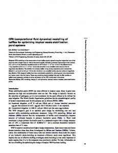
domain should be sufficiently large so that flow conditions at the model boundaries do not create artificial conditions within the region of interest. A sufficient amount of the upstream geometry must be included to achieve a fully developed flow field prior to the area of interest. Traditionally, the upstream boundary needs to be at least 5–10 times the characteristic length upstream from the area of interest, but should be farther upstream if there are bends, transitions, obstructions, or other changes in flow direction within this region. Figure 4 displays an example of a UV system that highlights the influence of providing sufficient upstream geometry to provide fully developed flow conditions at the area of interest. In this example, the area of interest is between two bends, where the reactor is located.

Figure 4

|


|

in press

|

2015

Placing the upstream boundary at 2.5 versus 10 diameters upstream from the reactor shows subtle differences in the velocity field at a vertical plane through the lamps. The pressure drop may be similar, but the differences in velocity will have a direct impact on the calculated dose from the lamps. Meshing A computational mesh is developed within the flow geometry. There are many available approaches to mesh generation and computational cell type. It is important that the mesh is sufficiently refined in the region of interest, and of sufficient quality overall to provide a converging

Sufficient upstream geometry is required for fully developed flow in the region of interest.

Uncorrected Proof 8

E. Wicklein et al.

|


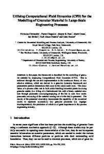
solution. In areas of the domain where solution variables are likely to have steep gradients, for example, a finer mesh is recommended to reduce propagation of numerical errors and promote convergence. The task of mesh generation is generally accomplished through the use of mesh-generating software that allows for definition of the model geometry, computational cell size, and grid density, and provides tools for grid quality analysis. Unstructured computational grids are the most common type, as they allow the greatest flexibility in defining the model domain and meshing properties. The mesh comprises computational cells that can range from 2D triangles to 3D, 20-faced polyhedral elements. Numerous meshing algorithms have been developed to match the mesh better with the surface and capture flow details. An ideal computational cell has flow entering and exiting perpendicular to the faces, with cell sides having similar edge lengths and equilateral angles between edges. Compound curved surfaces and transitions between various complex surfaces lead to cell deformations that reduce mesh quality and can lead to numerical diffusion errors. Key general mesh quality metrics include mesh skewness and length ratio, as shown in Figure 5. Skewness is a measure of how far the cell faces deviate from equilateral and should generally be below 0.9 for most solvers, particularly in the area of interest. The cell-length ratio is the comparison between the lengths of the side and should generally be minimized such that all sides are similar in length. As the length ratio increases, solution quality will diminish, particularly if flow is not travelling parallel to the longest cell dimension. There are cases where higher length ratios may be tolerated, such as in the boundary layer region, where flow generally does travel parallel to the longer length sides. Although modern computers have ever-increasing capabilities, a balance is always needed between overall mesh


|

in press

|

2015

resolution and computational efficiency to generate a solution in a reasonable amount of time. Mesh independence analysis is generally recommended to verify the solution is not dependent upon the number of nodes used to solve a given problem, i.e. the model solution changes with reducing the computational cell size (and increasing the overall cell count). A coarse grid may have a lower level of inherent stability (and higher degree of numerical diffusion), while a fine grid will be numerically more stable, but will require increased computational effort, both because of the increased degrees of freedom, but also because of an increased model stiffness (different order of magnitude in model process rates). Increasing the fineness of the mesh also imposes the need for smaller time steps to maintain stability for transient simulations. Consideration must be given also to the minimum number of computational cells across flow regions to maintain accuracy of the numerical scheme. For example, five cells as a minimum are required for 2nd order accurate solutions. The mesh should be finer in areas of interest and where sharp gradients may occur (e.g. inlet, outlets, free surface, near agitators …), and smoothly transition between finer and coarser mesh regions. For most wastewater applications the bulk flow region is of primary interest and this is where most wastewater process reactions typically occur. Therefore the flow details within the boundary layer are usually not of primary interest and consequently should be sufficiently refined for use of wall functions to determine the transition from no-slip at a wall to the free stream flow. It is recognized that modellers often do not run mesh independence studies for all problems due to resource constraints, particularly where previous or similar representative geometries have been analysed, or reasonable engineering judgment can be utilized to develop the model mesh. Thus, when reporting CFD results, the mesh type should always be noted as well as the overall cell count and a detailed image of the mesh should be provided. This is a prerequisite for judging the quality of the CFD exercise as mesh quality is critical for accurate solutions and subsequent interpretation of the results. Solver setup

Figure 5

|

Cell quality examples.

Once the mesh is developed, the model solver needs to be set up to calculate the CFD solution. In general, a double precision solver with second order discretization should be used for all wastewater problems. Many of the species modelled occur in low concentrations, implying the need for high numerical accuracy. Details of pressure-velocity

Uncorrected Proof 9

E. Wicklein et al.

|



|

in press

|

2015

WWT typically requires several phases: wastewater, suspended solids and gas phase in aerated zones. If biokinetic changes are to be modelled, dissolved species must also be introduced and could transition between phases. The model phases will need their physical properties applied, including density and viscosity as a minimum. Additional factors may also be required when supplemental energy (like mixing) is included in the solution.

turbulence models are available and routinely used. The selected model should be appropriate for the problems in question. There are numerous references that discuss the details of the various models (Versteeg & Malalasekera ; Wilcox ; Ferziger & Peric ). In current practice, two equation models such as k-ε and k-ε are most commonly used for wastewater modelling, although both computationally simpler and more complex models are sometimes used in some cases. Table 1 displays different types of turbulence models with advantages and disadvantages in their performance. Launder & Spalding () provide an early overview reference on turbulence models. The basic turbulence models commonly used in hydraulic engineering have been reviewed by the ASCE Task Committee () and Rodi ().

Turbulence models

Boundary conditions

Almost any CFD problem in wastewater flows will typically require a suitable approach to turbulence. A wide range of

The flow field computed by the CFD model is a direct function of the flow conditions applied at the domain

coupling scheme and equation discretion can be found in Patankar (), Versteeg & Malalasekera (), and Lomax et al. (). Multiphase models

Table 1

|

Turbulence model selection, advantages and disadvantages

Model

Advantages

Disadvantages

Two-Equation (standard k-ε, Renormalized Group (RNG) k-ε, Chen Kim k-ε and Realizable k-ε)

Simplest turbulence models that only require initial/boundary conditions

Have been found to perform poorly for the following cases:

Most widely tested models that have performed reasonably well for many types of flow conditions

• • • •

Second moment (Reynolds Stress Transport Model/Algebraic Stress Transport Model

Most general of traditional turbulence models that only require initial/boundary conditions More accurate representation of Reynolds stresses that better characterize the turbulent flow properties in wall jets flows with curved boundary layers or swirling flows rotating flows fully developed flows in non-circular ducts

• • • • DES

LES

A hybrid model that blends a two equation model near the walls with the LES model in the free stream More accurate for dynamic flow phenomenon than the simpler turbulence models Appropriate for complex free shear flows Used for turbulent boundary layers with high grid resolution at low Re

some unconfined flows flows with curved boundary layers or swirling flows rotating flows fully developed flows in non-circular ducts

Higher computing cost Has not been widely tested compared to the two equation models Has flow conditions that it has been found to behave poorly: axis-symmetric jets unconfined recirculating flows

• •

Has not been as widely tested as the two equation models Higher computing cost

Has not been widely tested compared to the two equation models Significantly higher computing cost

Uncorrected Proof 10

E. Wicklein et al.

|


boundaries, known as boundary conditions. Typical fluid flow boundaries include inlet boundaries, outlet boundaries, pressure boundaries, symmetry boundaries, and wall boundaries. Inlet boundaries provide a velocity or mass flow rate in the three vector components into or out of the model domain, as well as turbulence characteristics. Pressure boundaries have constant pressure and turbulence characteristics, and flow can move in or out of the domain. Outlet boundaries only allow flow to travel out of the domain, and may have no pressure constraints or turbulence constraints. Symmetry boundaries allow no vector component normal to the boundary. Wall boundaries are considered solid with no flow through the boundary. The wall boundary type can either be no slip (zero velocity) with a roughness component, or a slip wall with no roughness component. Typically, a wall function is used to approximate the transition from the zero velocity at the boundary through the boundary layer into the free stream. These wall functions model the effective drag from the roughness at the wall, without requiring the large number of computational elements required to resolve the flow field within the boundary layer. For wall boundary conditions, the no-slip condition (i.e., velocities equal to zero at the wall) is applied to all solid surfaces. At very small distances near the solid wall, a viscous sub-layer exists and is followed by an intermediate layer and turbulent core. In the viscous sub-layer, the flow is influenced by viscous forces and does not depend on free stream turbulent parameters. The velocity in this sub-layer only depends on the distance normal to the wall, fluid density, viscosity, and the wall shear stress. Typically, the viscous sub-layer is too thin to discretize and is therefore not included as a significant region in turbulence models in WWT reactors. However, the intermediate region, which includes effects of both the viscous sub-layer and the turbulent core, is more significant in size and requires more care in predicting the velocity and turbulence. The intermediate sub-layer is bridged by utilizing empirical wall functions to provide near-wall boundary conditions for the mean-flow and turbulence transport equations. The purpose of these empirical functions is to connect the wall shear stress to the dependent variables at the near-wall grid node. This grid node must lie outside this sub-layer and reside in the fully-turbulent zone. There are two types of wall function provided in commercial CFD codes: equilibrium log-law wall functions and non-equilibrium log-law wall functions. Non-equilibrium log-law wall functions should be used when there is turbulent transport of heat, and species at a reattachment point.


|

in press

|

2015

Reactions, energy, biokinetics and multiphase flows require additional boundary condition information. The additional parameters are typically added at the flow and wall boundary conditions and could include the wall and fluid temperature, species concentrations, or phase information. Steady vs dynamic The selection of whether to perform a steady-state or dynamic (transient, time-dependent) CFD simulation is a key stage in the process. A steady-state simulation uses an iterative scheme to progress to convergence, but persistent oscillations in the convergence residuals may indicate dynamic flow (transient) characteristic and the model may need to be performed as a time dependent simulation. Dynamic simulations also take much longer to compute, so the initial choice of a steady simulation is generally the most practical option, unless dynamic conditions are part of the problem objective, such as when the input variables are simply changing (e.g. diurnal flow, a cascading flow, or flows with changing salinity, temperature or influent composition.). A dynamic simulation approach can also be used to converge to the equivalent steady-state solution over time. Applying transient simulations can be very useful for multiphase applications, particularly biokinetic modelling when the interaction between multiple phases is complex. Convergence Numerical solution methods are typically solved iteratively, the convergence error being the difference between the calculated solution and exact solution (Wilcox 2000). Unfortunately, the model will typically not reach the exact solution; therefore metrics are needed to judge when the model is sufficiently converged. Commonly, the residual error, the sum of the differences between the currently iterated solution and the previously iterated solution for each cell and its nearest neighbours (or next-nearest neighbours in the case of 2nd order schemes) is the first measure. This difference should reduce over time, while satisfying the main criteria that the mass flow should remain continuous. Finally, the solution at discrete points should be stable (Wilcox 2000). Calibration and validation The core CFD model, if set up properly, should not require calibration to solve the fundamental fluid flow equations


E. Wicklein et al.

|


accurately for a single species single phase flow with appropriate boundary conditions and an adequate mesh, as the parameters used are based on physics or known properties, and hence are not contestable. However, there are uncertainties in many typical wastewater applications that may require some level of calibration. Submodels for scalar quantities (e.g. solids) often require empirical fits that are subject to many factors that cannot be isolated for a given problem without some local data. For example, settling velocities can be measured on site. Solids profiles can be measured under one condition and the model compared to the measured data. In some cases, modifications in the fit parameters for the empirical models can improve the prediction of local site performance of the model. In general, however, the focus of data-model comparison for CFD purposes is model validation rather than parameter estimation or calibration as it is preferable to measure parameters for empirical model development through dedicated controlled experiments. Data collection for validation is both time consuming and resource intensive as it typically requires advanced measurement techniques. Velocity measurements such as Acoustic Doppler Velocimetry or Laser Doppler Velocimetry (LDV) can be used. These require specific skills and expertise to conduct (Vanrolleghem et al. ) and have their limitations, e.g. the studied reactor should be relatively small and both water and reactor should be transparent (at least one wall for 2D observation) for LDV to be applicable. Additionally, spatial profiling of certain species within the reactor (e.g. solids concentration or dissolved oxygen) and reactive tracer methods have been used (Gresch et al. ; Liotta et al. ). Caution should be exercised when using a visual inspection of 2–3D graphs of experimental data and model predictions as this approach is subjective. A quantitative approach that makes a numerical comparison of model error using an error evaluation technique is preferred. Validation by solids and dye profiling (tracer test) is also a relatively inexpensive and well-documented procedure and can be used for validation of solids transport modelling for many WWT applications (Bender & Crosby ). Other non-reactive tracers can be used, such as Lithium Chloride, which is relatively expensive and needs special analysis equipment (e.g., atomic absorption) to measure low concentrations (mg/L) but yield good results. There are two main kinds of methods to simulate residence time distributions (RTD) with CFD: Lagrangian particle tracking (Thyn et al. ; Stropky et al. ) and solving the transport equation for a passive tracer with a scalar representing the tracer


|

in press

|

2015

concentration (Talvy et al. ; Zhang et al. ). The second method is sensitive to numerical diffusion, so care is required when it is used. However, if the subsequent goal is to implement biokinetics, the best numerical RTD approach is to use the scalar method, because simulations that include biokinetics also utilize the transport equation (see further), and it is important to create similar conditions for both CFD-RTD and the subsequent integrated CFD biokinetics model (Le Moullec et al. ). Caution should be used with tracer testing as similar RTD could be produced for multiple internal vessel geometries. Therefore, these tests should be used in conjunction with other methods when possible. It is important to note that the hydrodynamics depends not only on the shape and size of reactors and physical properties of the liquid, but also the energy engaged in the process and the flow rates (Potier et al. ). Hence, reactor hydrodynamics strongly vary over the course of the day, since liquid flow rate fluctuates significantly. Current and future added value of CFD The current portfolio of CFD components in the field of WWT is illustrated in Figure 6. Next to ‘plain CFD’ which simply computes (single phase) flow patterns, different ingredients can be added resulting in an ‘extended CFD’ approach. Some of these are more straightforward than others and are recommended to be used as state of the art (e.g. density, soluble transport). The efficiency of others

Figure 6

|

Current portfolio of CFD models in the field of WWT.


E. Wicklein et al.

|


has not yet reached consensus and is being debated in literature (e.g. rheology, solids transport, flocculation). These are case specific and should be used with caution and, if possible, with calibration and validation to advance the state of the art. A key potential opportunity is application of previously developed components in general wastewater modelling to enhance use of CFD. An example of this is application of the double exponential settling function to solids sedimentation in a CFD context (Takács et al. ). To date, CFD models have primarily been used for design analysis and troubleshooting, mainly due to the computational effort. However, more frequent use of CFD and the accumulation of knowledge should increasingly allow for optimization of design and operation, even in shorter time frames. This has already been applied to secondary sedimentation (e.g., Griborio & McCorquodale ; Xanthos et al. ) and mixing (Samstag et al. ), but will also be true for other processes. Optimization can both be in terms of process performance (such as improved conversion through ‘smart’ mixing and improved removal of a particular species) as well as in energy reduction (e.g. smarter location and operation of impellers, aerators and sensors serving as controller inputs (Rehman et al. b)). CFD can be used to develop biokinetic models of biological treatment reactors based on fully realized velocity fields in the reactor tanks rather than on simplified models such as the tanks in series (TIS) modelling approach typically used in the IWA Activated Sludge Models (Hangos & Cameron ) and other commercial models in wide use today. Care must be taken when incorporating biokinetic models as some have been derived with assumed mixing conditions. In some cases, the biokinetics have been ‘calibrated’ by forcing a TIS model to match available data through arbitrarily adjusting the model parameters within the degrees of freedom, neglecting the fact that TIS may miss key hydraulic details in the system (Alvarado et al. ). Generally, biological species (dissolved oxygen, ammonia, nitrates etc.) can be introduced as user defined scalars in the solver. Biological reactions then provide the production and/or consumption of these species, which are used as source/sink terms in the transport equations for each species (Rehman et al. a). In multiphase systems, mass transfer between the phases can also be incorporated either using the user defined scalars or species transport within the solver. Efforts to combine CFD with ASM models are ongoing as well (e.g. Le Moullec et al. b, ; Sobremisana et al. ) Finally, next to the use of CFD as a stand-alone tool in system optimization, a second route will be to use CFD as


|

in press

|

2015

a means to build up knowledge which can then serve to improve the simpler models we are currently using. The first examples have been reported in literature where CFD models are used to build somewhat more detailed mixing models called ‘compartmental models’ (compared to the current practice of tanks-in-series) (Le Moullec et al. a, ; Alvarado et al. ). In this way CFD models clearly have a complementary and supporting role to play in WWT modelling and by no means will replace the traditional ones in the near future. On the contrary, they are an important tool to extend our knowledge further and exploit the power of mathematical modelling for WWT systems as recently corroborated by Laurent et al. ().

CONCLUSION The potential for CFD in WWT applications is great. However, to date this potential has not been fully exploited. One of the reasons for this, next to lack of training for practitioners, is lack of guidance with respect to GMP for water and wastewater applications. GMP should cover the complete process from objective definition to problem solution and visualization of results. In this paper we have tried to outline briefly the principal features of GMP for WWT. This should allow modellers new to the application of CFD in the wastewater field to conduct a CFD studies. This will increase trust in these models and allow the exploitation of their full potential in the future.

ACKNOWLEDGEMENTS This work has been completed as part of the work of the IWA Working Group on CFD.

REFERENCES Alvarado, A., Vedantam, S., Goethals, P. & Nopens, I.  Compartmental models to describe hydraulics in full-scale waste stabilization ponds. Water Research 46 (2), 521–530. Amato, T. & Wicks, J.  The practical application of computational fluid dynamics to dissolved air flotation, water treatment plant operation, design and development. Journal of Water Supply: Research and Technology-AQUA 58 (1), 65–73. American Institute of Aeronautics, Astronautics (AIAA)  Guide for the Verification and Validation of Computational Fluid Dynamics Simulations. AIAA G-077–1998, Reston, VA, USA.


E. Wicklein et al.

|


ASCE Task Committee  Turbulence modelling of surface water flow and transport: part I, II, III, IV, V, Task committee on turbulence models in hydraulic computations. Journal of Hydraulic Engineering 114 (9), 970–1073. Bender, J. & Crosby, R.  Hydraulic Characteristics of Activated Sludge Secondary Clarifiers, Project Summary. US EPA 600/S2-84-131, USA. Brannock, M., Wang, Y. & Leslie, G.  Mixing characterisation of full-scale membrane bioreactors: CFD modelling with experimental validation. Water Research 44 (10), 3181–3191. Bridgeman, J.  Computational fluid dynamics modelling of sewage sludge mixing in an anaerobic digester. Advances in Engineering Software 44, 54–62. Casey, M. & Wintergerste, T. (eds.) 2000 Special Interest Group on ‘Quality and Trust in Industrial CFD’ Best Practice Guidelines, Version 1. ERCOFTAC Report. Crowe, C., Sommerfeld, M. & Tsuji, Y.  Multiphase Flows with Droplets and Particles. CRC Press, Boca Raton, LA, USA. De Clercq, B.  Computational Fluid Dynamics of Settling Tanks: Development of Experiments and Rheological, Settling and Scraper Submodels. PhD thesis, Ghent University, Belgium. Eshtiaghi, N., Markis, F., Yap, S. D., Baudez, J. C. & Slatter, P.  Rheological characterization of municipal sludge: a review. Water Research 47 (15), 5493–5510. Ferziger, J. H. & Periˇc, M.  Computational Methods for Fluid Dynamics. Springer, Berlin, Germany. Gresch, M., Braun, D. & Gujer, W.  Using reactive tracers to detect flow field anomalies in water treatment reactors. Water Research 45 (5), 1984–1994. Griborio, A. & McCorquodale, J. A.  Optimum design of your center well: Use of a CFD model to understand the balance between flocculation and improved hydrodynamics. In: Proceedings of the Water Environment Federation 79th Annual Conference and Exposition, Dallas, TX, USA, October 21–26, 2006. Guerts, J. B.  Elements of direct and large-eddy simulation. Edwards Inc., Philadelphia, USA. Hangos, K. M. & Cameron, I. T.  Process Modelling and Model Analysis, Volume 4. Academia Press, London, UK. Henze, M., Gujer, W., Mino, T. & van Loosdrecht, M. C. M.  Activated Sludge Models ASM1, ASM2, ASM2d and ASM3. Scientific & Technical Report No 9, IWA Publishing, London, UK. Ho, C. K., Khalsa, S. S., Wright, H. B. & Wicklein, E.  Computational Fluid Dynamics Based Models for Assessing UV Reactor Design and Installation. Water Research Foundation, Denver, CO, USA. Khan, L. A., Wicklein, E. A. & Teixeira, E. C.  Validation of a three-dimensional computational fluid dynamics model of a contact tank. Journal of Hydraulic Engineering 132 (7), 741–746. Launder, B. E. & Spalding, D. B.  Lectures in Mathematical Models of Turbulence. Academic Press, London, UK and New York, USA. Laurent, J., Samstag, R. W., Ducoste, J. M., Griborio, A., Nopens, I., Batstone, D. J., Wicks, J. D., Saubers, S. & Potier, O. 


|

in press

|

2015

A protocol for the use of computational fluid dynamics as a supportive tool for wastewater treatment plant modeling. Water Science and Technology 70 (10), 1575–1584. Le Moullec, Y., Potier, O., Gentric, C. & Leclerc, J. P.  Flowfield and residence time distribution simulation of a cross-flow gas–liquid wastewater treatment reactor using CFD. Chemical Engineering Science 63 (9), 2436–2449. Le Moullec, Y., Gentric, C., Potier, O. & Leclerc, J. P. a Comparison of systemic, compartmental and CFD modelling approaches: application to the simulation of a biological reactor of wastewater treatment. Chemical Engineering Science 65 (1), 343–350. Le Moullec, Y., Gentric, C., Potier, O. & Leclerc, J. P. b CFD Simulation of the hydrodynamics and reactions in an activated sludge channel reactor of wastewater treatment. Chemical Engineering Science 65 (1), 492–498. Le Moullec, Y., Potier, O., Gentric, C. & Leclerc, J. P.  Activated sludge pilot plant: comparison between experimental and predicted concentration profiles using three different modelling approaches. Water Research 45 (10), 3085–3097. Li, S., Lai, Y., Weber, L., Silva, J. M. & Patel, V. C.  Validation of a three-dimensional numerical model for water-pump intakes. Journal of Hydraulic Research 42 (3), 282–292. Liotta, F., Chatellier, P., Esposito, G., Fabbricino, M., Van Hullebusch, E. D. & Lens, P. N. L.  Hydrodynamic mathematical modelling of aerobic plug flow and Non-ideal flow reactors: a critical and historical review. Critical Reviews in Environmental Science and Technology 44 (23), 2642–2673. Liu, X. & Garcia, M. H.  Computational fluid dynamics modeling for the design of large primary settling tanks. Journal of Hydraulic Engineering 137 (3), 343–355. Lomax, H., Pulliam, T. & Zingg, D.  Fundamentals of Computational Fluid Dynamics. Springer, Berlin, Germany. Markis, F., Baudez, J. C., Parthasarathay, R., Slatter, P. & Eshtiaghi, N.  Rheological characterisation of primary and secondary sludge: impact of solids concentration. Chemical Engineering Journal 253, 526–537. McCorquodale, J. A., Griborio, A., Li, J., Horneck, H. & Biswas, N.  Modeling a retention treatment basin for CSO. Journal of Environmental Engineering 133 (3), 263–270. Nopens, I., Wicks, J., Griborio, A., Samstag, R., Batstone, D. & Wicklein, E.  Computational fluid dynamics (CFD): what is good CFD-modelling practice and what can be the added value of CFD models to WWTP modelling? In: Proceedings of the 85th Annual Conference and Exposition, New Orleans, LA, USA, September 29- October 3, 2012. Patankar, S. V.  Numerical Heat Transfer and Fluid Flow. Hemisphere Publishing Corporation, Taylor & Francis Group, New York, USA. Potier, O., Leclerc, J. P. & Pons, M. N.  Influence of geometrical and operational parameters on the axial dispersion in an aerated channel reactor. Water Research 39 (18), 4454–4462. Ratkovich, N., Horn, W., Helmus, F. P., Rosenberger, S., Naessens, W., Nopens, I. & Bentzen, T. R.  Activated


E. Wicklein et al.

|


sludge rheology: a critical review on data collection and modelling. Water Research 47 (2), 463–482. Rehman, U., Maere, T., Amerlinck, A., Arnaldos, M. & Nopens, I. a Hydrodynamic–biokinetic model integration applied to a full-scale WWTP. In: Proceedings of the IWA World Water Congress & Exhibition, Lisbon, Portugal, September 2014. Rehman, U., Vesvikar, M., Maere, T., Guo, L., Vanrolleghem, P. A. & Nopens, I. b Effect of Sensor Location on Controller Performance in a Wastewater Treatment Plant. Water Science and Technology 71 (5), 700–708. Roache, P. J.  Qualification of Uncertainty in Computational Fluid Dynamics. Annual Review of Fluid Mechanics 29, 123–160. Rodi, W.  Turbulence Models and their Application in Hydraulics–A state-of-the-art review, 3rd edn. International Association for Hydraulic Research, Balkema, Rotterdam, Brookfield. Samstag, R. W., Wicklein, E. W., Reardon, R. D., Leetch, R. J., Parks, R. M. & Groff, C. D.  Field and CFD Analysis of Jet Aeration and Mixing. In: Proceedings of the 84th Annual Water Environment Federation Technical Conference & Exposition, New Orleans, LA, USA, October, 2012. Sobremisana, A. P., Ducoste, J. J. & de los Reyes III, F. L..  Combining CFD, Floc Dynamics and Biological Reaction Kinetics to Model Carbon and Nitrogen Removal in Activated Sludge System. In: Proceedings of the 83rd Annual Water Environment Federation Technical Conference and Exposition, Los Angeles, CA, USA, October 15–19, 2011. Spalart, P. R.  Detached Eddy simulation. Annual Review of Fluid Mechanics 41, 181–202. Stropky, D., Pougatch, K., Nowak, P., Salcudean, M., Pagorla, P., Gartshore, I. & Yuan, J. W.  RTD (residence time distribution) predictions in large mechanically aerated lagoons. Water Science and Technology 55 (11), 29–36.


|

in press

|

2015

Takács, I., Patry, G. G. & Nolasco, D.  A dynamic model of the clarification-thickening process. Water Research 25 (10), 1263–1271. Talvy, S., Cockx, A. & Line, A.  Modeling hydrodynamics of gas–liquid airlift reactor. A.I.Ch.E. Journal 53 (2), 335–353. Thyn, J., Ha, J. J., Strasak, P. & Zitny, R.  RTD Prediction, modelling and measurement of gas flow in reactor. Nukleonika 43 (1), 95–114. Vanrolleghem, P. A., De Clercq, B., De Clercq, J., Devisscher, M., Kinnear, D. J. & Nopens, I.  New measurement techniques for secondary settlers: a review. Water Science and Technology 53 (4–5), 419–429. Versteeg, H. K. & Malalasekera, W.  An Introduction to Computational Fluid Dynamics. Longman, London, UK. Wicklein, E. A. & Samstag, R. W.  Comparing Commercial and Transport CFD Models for Secondary Sedimentation. In Proceedings of the 81st Annual Water Environment Federation Technical Exhibition and Conference, Orlando, FL, USA, October, 2009. Wilcox, D. C.  Turbulence Modeling for CFD, 2nd ed. DCW Industries, La Canada, Canada. Wu, B. & Chen, S.  CFD Simulation of non-newtonian fluid flow in anaerobic digesters. Biotechnology Engineering 99 (3), 700–711. Xanthos, S., Gong, M., Ramalingam, K., Fillos, J., Deur, A., Beckmann, K. & McCorquodale, J. A.  Performance assessment of secondary settling tanks using CFD modelling. Water Resources Management 25 (4), 1169–1182. Zhang, L., Pan, Q. & Rempel, G. L.  Residence time distribution in a multistage agitated contactor with Newtonian fluids: CFD prediction and experimental validation. Industrial and Engineering Chemistry Research 46 (11), 3538–3546.

First received 5 May 2015; accepted in revised form 23 October 2015. Available online 9 November 2015