guidance on the use of computational fluid dynamics for modelling ...

GUIDANCE ON THE USE OF COMPUTATIONAL FLUID DYNAMICS FOR MODELLING BUOYANCY DRIVEN FLOWS Malcolm J. Cook; Kevin J. Lomas Fundamentals - Air Flow

GUIDANCE ON THE USE OF COMPUTATIONAL FLUID DYNAMICS FOR MODELLING BUOYANCY DRIVEN FLOWS Malcolm J. Cook BSc MSc GIMA & Kevin J. Lomas PhD CEng MCIBSE MInstE Institute of Energy & Sustainable Development, De Montfort University, The Gateway, Leicester, LE1 9BH, UK http://www.iesd.dmu.ac.uk

employed. The results of these experiments compared favourably with the theory. The CFD approach is being used to explore the same idealistic conditions.

ABSTRACT Buoyancy driven flows have always been, and still are, difficult to model using CFD programs. Much validation work is required along with guidelines for the CFD practitioner about how to model such flows. This paper makes a contribution to these two areas by considering buoyancy driven displacement ventilation in a very simple geometry.

Buoyancy driven flows are notoriously difficult to model using CFD techniques for the following reasons: small driving forces lead to numerical instabilities; there is uncertainty regarding how to accurately model turbulence; and the flow is implicitly specified (i.e. sources of buoyancy are specified from which the program must calculate a velocity field). Consequently, much validation work is needed to evaluate the ability of these codes to model such flows.

The nature of buoyancy driven displacement ventilation is briefly described and guidance offered on how to represent the problem in a CFD program. Simulations were carried out using two eddy viscosity turbulence models. The results show good qualitative agreement with experimental data and analytical results but small discrepancies in some of the quantitative results.

It is the intention of this paper to offer guidance on how to model buoyancy driven flows and the accuracy which can be expected from a commercial CFD package. The simulations reported here comprise simple geometries with a single source of buoyancy, but it is hoped that the conclusions drawn and the experience gathered can be used in modelling more complex, real buildings.

INTRODUCTION Buildings must be provided with adequate ventilation. Environmental concerns together with demands for energy efficiency are prompting designers to investigate natural ventilation as an alternative to mechanical ventilation or full air conditioning. Buoyancy driven displacement ventilation is proving to be a popular approach, and it is the modelling of this phenomenon, using Computational Fluid Dynamics (CFD), that is addressed in this paper.

THEORY OF BUOYANCY DRIVEN DISPLACEMENT VENTILATION A good example of a buoyancy driven flow is displacement ventilation in which use is made of the buoyancy forces produced by naturally occuring heat sources such as occupants and equipment (e.g. computer terminals, projector units, etc).

Buoyancy driven displacement ventilation occurs when thermal plumes produced above occupants and equipment cause a layer of warm, buoyant air to form close to the ceiling of the space. This layer drives a flow through high-level openings and causes fresh, ambient air to be drawn in at low level. A prominent feature of this flow is the formation of a horizontal interface separating the warm, buoyant air above, from the ambient, cooler air below. A theory for this type of flow was described by Linden et al. (1990) who considered displacement ventilation of a simple rectangular box. To visualise these flows, the salt bath modelling technique was

The theory for this type of flow was elucidated by Linden et al. (1990) who considered displacement ventilation of a simple rectangular box (fig. 1). The heat source produces a rising plume which entrains fresh (ambient) air taking it upwards into the upper region of the space where it is recirculated. As more and more light air accumulates in the upper region of the space, the rising plume begins to entrain this lighter air until a steady-state is achieved (fig. 1), in which a constant interface forms (at y = h ) separating the dense, cool

1

air below the interface from the warmer, buoyant air above. In the steady-state, the layer of warm, buoyant air drives a flow through the upper openings since the hydrostatic pressure difference between the top and bottom of the layer is smaller inside the space than between the same heights outside the space. This causes fresh air to be drawn in through the lower openings.

and brine injected to represent the effects of a heat source.

DETAILS OF THE CFD PACKAGE The CFD package used for this work was CFX-F3D (1996). The code solves the conservation equations for mass, momentum and energy (enthalpy): ∂ ∂ ρu j φ − ∂x j ∂x j

(

y=H

)

 ∂φ   Γφ  = Sφ  ∂x j 

(3)

The source terms and diffusion coefficients are given in table 1 for the variable φ. All transient terms have been omitted since the work sought steady-state solutions.

y=h

Table 1. Terms in the governing equations when using an eddy viscosity turbulence model. φ

Γφ

Momentum

1 ui

0 µ + µT

Enthalpy

He

λ µ + T CP σ He

Conservation

y=0

Heat Source

equation Mass

Figure 1. Steady displacement ventilation flow in a box containing a constant heat source (arrows show direction of flow), after Linden et al. (1990) Linden et al. (1990) used the plume theory of Morton et al. (1956) to derive an expression for the interface height (eq. 1) by equating volume and buoyancy fluxes in the plume with those through the inlets. ( )  A = C 3/ 2   2 H  1 − Hh  *

h H

5

0 ∂ ∂x j

 ∂u   − p0 δ ij + µ eff i  + ρgi ∂x j  

0

p 0 is a ‘modified’ pressure given by

p0 = p +

1/ 2

(1)

2 ρk − ρBref gi xi . 3

(4)

where ρBref is a buoyancy reference density. Turbulence modelling is a crucial aspect of all CFD modelling, but is particularly important in buoyancy driven flows in which the buoyancy forces increase turbulent activity. This paper considers two models. The first is the industry standard k − ε model of Launder and Spalding (1974) in which transport equations for k and ε are solved as follows:

where A* is an effective opening area defined as a u al A* = (2) 1/ 2 2 1 / 2(au / c + al2 )

[

Sφ

]

where: au al c

= total area of upper openings; = total area of lower openings; and = momentum theorem constant (= 1 throughout this work), 9 6 and C = 5 α( 10 α )1/ 3 π 2 / 3 is a constant dependent upon the entrainment constant α . The entrainment constant is an empirical value and can be thought of as a proportionality constant relating inflow velocity at the edge of the plume with the upward velocity on the axis of the plume. Measuring α is very difficult and several authors have suggested values (e.g. Morton et al. (1956), Baines et al. (1968)). The value used thoughout this work is that used by Linden et al. (1990), ( α = 0.1 ).

∂ ∂ ρu jk − ∂x j ∂x j

(

)

∂ ∂ ρu j ε − ∂x j ∂x j

(

)

 µ  ∂k    µ + T   = P + G − ρε σ k  ∂ x j  

(5)

 µ  ∂ε  ε ε 2 (6)   µ + T   = C1 P − C2ρ σ ε  ∂x j  k k 

where C1 = 1.44 and C2 = 1.92 are empirical constants. P and G represent the production of turbulent kinetic energy due to shear stresses and buoyancy respectively: P = µ eff

Linden et al. (1990) verified their theoretical predictions using the salt bath modelling technique in which perspex models are inverted in fresh water

∂ui ∂x j

G=

2

 ∂ui ∂u j    ; and +  ∂x j ∂xi  µ eff σT

βg j

∂T . ∂x j

where σ T is the turbulent Prandtl number for k or ε depending upon which equation is being considered.

at the same position, thus producing a more readily understood solution field. All the governing equations are discretised using hybrid differencing (except the mass conservation equation where central differencing is always used). The finite volume solution method is used (see Versteeg et al. (1995)), and pressure and velocity are coupled using the SIMPLEC algorithm with Rhie-Chow interpolation (Rhie and Chow (1983)) to prevent decoupling of pressure and velocity due to the co-located grid. The following (default) underrelaxation factors were used: momentum, 0.65; mass, 1.0; enthalpy, 1.0; k, 0.7; and ε, 0.7. These are similar to those used in most CFD codes.

The second is the more recent RNG k − ε model based on Renormalised Group (RNG) theory established by Yakhot and Orszag (1992). This model assumes the same form of the k and ε equations as the model of Launder and Spalding (1974) but uses RNG theory to calculate the constants. The constants are represented in CFXF3D as follows. C1 is replaced with C1 − C1 RNG where

C1 RNG

 P η=   µT 

1/ 2

 η η1 −  η0   = , (1 + β1η3 )

Buoyancy is modelled using the Boussinesq approximation (see Turner (1973)) in which density is assumed to be constant except in the momentum equation where it is written

( (

k , β1 = 0.015 and η0 = 4.38 . ε

ρ = ρBref 1 − β T − TBref

(7)

This gives rise to the buoyancy term in the modified The Boussinesq pressure, p 0 in table 1. approximation is only applicable in flows where the density differences are small. Those that occur in buildings due to temperature variations are sufficiently small.

C1 = 1.42, and C2 = 1.68.

The models differ in the way the constants are derived. In the standard k-ε model, all constants are found empirically. This has the disadvantage of the constants only being applicable to the types of flow from which they were derived. However, good results have been obtained for many air flow applications using this model. In the RNG model, the constants are derived mathematically such that the constants are valid for a very wide range of flow types including both high and low Reynolds number flows. It is interesting to note that the RNG theory gives rise to a new rate-of-strain term in the ε equation. This equation has long thought to have been responsible for inaccuracies in the standard k-ε model when large deformormation forces are present (Versteeg et al. (1995)).

Three types of boundary condition are used in this investigation: WALL boundaries; PRESSURE boundaries; and SYMMETRY PLANE boundaries. WALL boundary conditions are placed at fluid-solid interfaces and enable the specification of velocities (normally zero), heat fluxes, and temperatures. Conventional wall functions are imposed at WALL boundaries (Versteeg et al. (1995)). Fluid may flow into or out of the domain across a PRESSURE boundary. If fluid flows into the domain, Neumann conditions (i.e. zero normal gradient) are imposed on velocity and turbulence quantities, and values assigned explicitly to pressure and temperature (Dirichlet conditions). When fluid flows out of the domain across a PRESSURE boundary, Dirichlet conditions are imposed on pressure, and Neumann conditions on all other variables.

In both models, the eddy viscosity, µ T is calculated using µ T = ρCµ

))

k2 ε

0.09 (standard k − ε ) where: Cµ =  0.085 (RNG k − ε )

At SYMMETRY PLANE boundaries, all variables are set to be mathematically symmetric, except the component of velocity normal to the boundary which is anti-symmetric.

CFX is a multiblock code in which one or more topologically rectangular blocks are ‘glued’ together to form the geometry. Variables are solved for at cell centres (a co-located grid) rather than the more traditional approach which uses a staggered grid. The co-located grid has the simple advantage of having both velocities and scalar quantities located

REPRESENTATION IN THE CFD MODEL In order to evaluate the ability of the CFD code to model displacement ventilation, a simple case was

3

defined similar to that in figure 1. The space was 5.1m wide, 2.55m high and 1m deep with upper and lower openings to the ambient air at 18°C. The flow was driven by a point source of buoyancy placed in the centre of the floor. Both the source strength and the opening areas were varried.

(7)). By considering the behaviour of equation (4) at the pressure boundary, the following is obtained (by substituting eq. (7) into eq. (4)):

Accurate modelling of the flow as it passed through the openings was considered important due to the loss in pressure head, or discharge, suffered by the flow as it expands and contracts. Therefore, instead of specifying boundary conditions at the openings, the flow through the openings was modelled explicitly by extending the computational domain beyond the room and specifying PRESSURE boundaries at some distance away. How much of the exterior to model was investigated in detail in Cook (1997), where a sensitivity analysis showed that extra space above and below the room (fig. 2) was sufficient.

At the PRESSURE boundary, in the absence of any local temperature gradient, p0 should equal 2 due to an extended Boussinesq 3 ρk − ρgi x i , relationship (see Versteeg et al. (1995)). In order for this to be so when p = 0 , the buoyancy reference temperature should be set equal to the temperature on the pressure boundary, i.e. the ambient temperature (see eq. (8)). Specifying any other temperature would generate an additional, unrealistic pressure force.

p0 = p +

(

)

(8)

There exists a disadvantage of using external pressure boundaries such as those used here (fig. 2). There is a tendency, in all CFD codes, to overpredict entrainment across these boundaries (early simulations showed unrealistically high velocities predicted in the z-direction in the exterior). This occurs because there is nothing in theory to stop the flow from doing this (Newton’s laws of motion). Thus a high velocity flow across these boundaries does indeed satisfy the governing equations. The problem is overcome simply by specifying WALL boundary conditions where this is a problem, i.e. at the high and low z faces in this case.

WALL boundary: u = 0, Q = 0 2.55m PRESSURE boundary: p = 0, T=18C

WALL boundary: Q = 200W (total across symmetry plane)

2.55m

2 ρgi xi ρk − 3 1 − β T − TBref

SYMMETRY PLANE boundary

It is common practice to force numerical symmetry in problems that are geometrically symmetric by means of a symmetry plane (fig. 2). This not only reduces computational time, but in this case aids convergence by ensuring that the development of the plume is uninhibited by any unbalanced lateral forces that may arise during the solution proceedure.

2.55m

y z 1.0m

x 2.55m

The mesh used in this investigation is shown in figure 3. It was found (Cook 1997) that further mesh refinement did not change the governing parameters of the flow, i.e. interface height and change in temperature across the interface. Accurate values for ∆T across the interface could be obtained using a coarser mesh. However, this produced a more diffuse stratification making it difficult to measure the interface height accurately.

Figure 2. Geometry and boundary conditions used in the simulations The distance of the PRESSURE boundaries from the room were such that any greater distance produced no further change in the flow inside the box, i.e. h / H . The value assigned to pressure at all PRESSURE boundaries was p = 0 . This was possible since in incompressible flows, pressure is arbitrary to within an additive constant, and the hydrostatic pressure difference is automatically taken care of in the momentum equation (see modified pressure (eq. (4)).

In order to monitor the progress of the solution proceedure it is necessary to define a monitoring point. The location of this point should be selected such that it provides the user with as much (useful) information as possible. For example, there would be little to be gained in placing it close to the heat source since this area is likely to converge with little difficulty as it is close to the driving force. Similarly it would be inadvisable to place it in the

When prescribing a value for p at a PRESSURE boundary in a buoyancy driven flow, consideration must be given to the buoyancy reference density (eq. (4)), or the buoyancy reference temperature (eq.

4

type of under-relaxation which reflects the time scale over which the flow evolves. Instead of specifying just one under-relaxation factor for each equation, false time-stepping enables underrelaxation factors to be specified in each cell in terms of a pseudo time-step, ∆t , and the volume of that particular cell. This enables much more specific under-relaxation factors to be specified. The only difficulty lies in deciding what values to set for ∆t . It was found by Cook (1997) that false time-steps of 0.1s on the two momentum equations eliminated the oscillations on all the variables. It is useful to note that this is approximately equal to the smallest cell size in the domain ([smallest cell 1/2 area] ) divided by the maximum velocity in the domain. Therefore, using the non-converged solution with default under-relaxation as an approximation to the converged result, an estimate could be found for ∆t . It should be noted that ∆t is only used to control the iteration proceedure, it is not unique in determining the final result and only needs to be accurate to within the same order of magnitude.

core of a recirculation zone since this may take a very long time to reach convergence. In the simulations reported here, the monitoring point was located in the centre of the upper opening.

Figure 3. Mesh density used in all simulations ( 40 × 90 × 16)

Under-relaxation and false time-stepping have the effect of reducing the amount by which a variable changes between iterations. This slows down the rate of convergence as more iterations are needed. Consequently, in order to minimise run times, it was decided to begin the simulation using default underrelaxation and to ‘switch on’ false time-stepping when the residuals had stopped falling, i.e. when the iteration proceedure had produced the best solution possible using the default under-relaxation factors. Convergence was achieved for both turbulence models by running for about 1000 iterations followed by about 2000 iterations, although the residuals were slightly higher for the RNG k − ε model compared with those for the standard k − ε model.

RESULTS In order to ensure that the mathematical model defined in the CFD code has been satisfactorily solved, one must identify some convergence criteria. An obvious criterion is that the values of the variables ( u i , p, k, ε, and He ) are constant to within a very small tolerance, say 0.01%. This is a neccesary condition but is not sufficient. Although the variables may be changing only very slightly, they could in fact be a long way from satisfying the governing equations. Consequently a convergence criterion is required on the residuals (the errors between the left and right hand sides of the discretised governing equations) to ensure they are sufficiently small. A suitable condition in this work is that the enthalpy residual (in watts) is small when compared with the total heat entering the domain (of order 1%, say).

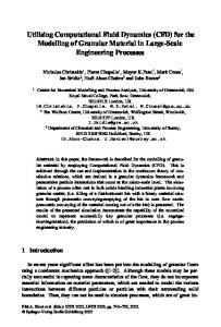
The resulting flow pattern (figs. 4, 5, 6 and 7) agreed favourably with the theoretical and experimental predictions of Linden et al. (1990). A rising plume forms above the heat source and produces stratification in the box. An interface forms across which there is a sharp change in temperature, and a flow is driven through the openings. When comparing the results showing the effects of various opening sizes, it can be seen that the RNG k − ε model gives a better prediction of the interface height than the standard k − ε model (fig. 8). This is thought to be due to the RNG model predicting a narrower plume than the k − ε model (c.f. figs. 4 and 5). The plume in figure 5 has to rise to a greater height before its volume flow rate matches that through the openings upon which it collapses and forms the interface. The narrower

In the simulations reported here, constant variables at the monitoring point could not be obtained using the default solution technique and under-relaxation factors. The enthalpy residual was too high and there were oscillations on all the variables. In an attempt to eliminate the oscillations, the amount by which a variable changed between subsequent iterations was reduced. This was done by imposing tighter under-relaxation, i.e. reducing the underrelaxation factors. However, convergence could still not be achieved. Another type of underrelaxation is false time-stepping. This is a particular

5

In all flow field figures, a vector of length 1cm corresponds to a flow speed of 0.3m/s.

21.25C 21.25C

18.5C

18.5C

Figure 4. Flow pattern predicted using standard k − ε turbulence model (total heat input = 200W, A* / H 2 = 0.0304)

Figure 5. Flow pattern predicted using RNG k − ε turbulence model (total heat input = 200W, A* / H 2 = 0.0304)

28.5C 21.5C

18.25C

18.75C

Figure 6. Flow pattern predicted using RNG k − ε turbulence model (total heat input = 200W, A* / H 2 = 0.0304) showing plane x = 0.2 m

Figure 7. Flow pattern predicted using RNG k − ε turbulence model (total heat input = 1000W, A* / H 2 = 0.0304)

6

plume suggests that the RNG k − ε model predicted a smaller rate of entrainment into the plume.

solve the governing equations. In these simulations, it was noted that the RNG k − ε model produced higher numerical errors (residuals) in the enthalpy equation than the standard k − ε model. The RNG k − ε model is still a new technique and very little validation has been carried out. Small changes in how the RNG k − ε technique is implemented may still be required, and this will be the subject of further investigation.

The work of Linden et al. (1990) concluded, amongst other things, that the height of the interface is independent of the source strength. Increasing the source strength only has the effect of inducing higher velocities and producing a larger temperature difference across the interface. CFD results for source strengths of 200W and 1000W verified these points (c.f. figs. 5 and 7).

ACKNOWLEDGEMENTS This work formed part of the first named author’s PhD work undertaken at De Montfort University. The authors wish to acknowledge the advise received from Dr. G. Whittle (Simulation Technology Ltd.) and Dr. P. Linden (University of Cambridge).

1.0 0.9 0.8

Theoretical prediction of Linden et al. Experimental results of Linden et al. CFX 4 (k−e model) CFX 4 (RNG k−e model)

0.7 0.6 h/H 0.5 0.4

REFERENCES

0.3

Baines, W. D. and Turner, J. S. “Turbulent Buoyant Convection from a Source in a Confined Region”, J. Fluid Mechanics 37, pp.51-82, 1968

0.2 0.1 0.0 0.00

0.01

0.02

0.03 * 2 A /H

0.04

0.05

Computational Fluid Dynamics Services, (AEA Harwell), “CFX 4.1 Flow Solver User Guide”, pp.263-350, 1995

0.06

Cook, M. J., “PhD Thesis”, in press, 1997

Figure 8. Variation of interface height with effective opening area for both turbulence models, using a heat source of 200W

Linden, P. F., Lane-Serff, G. F., and Smeed, D. A. “Emptying Filling Boxes: The Fluid Mechanics of Natural Ventilation”, J. Fluid Mechanics 212, pp.309-335, 1990

CONCLUSIONS This work has verified that bouyancy driven flows are difficult to model and tight control is required in the solution process of the equations. This is best done by use of under-relaxation factors which are both cell dependent and pseudo time dependent. Despite this, favourable qualitative agreement was obtained between the CFD results and the theoretical and experimental work of Linden et al. (1990) for a simple space undergoing buoyancy driven displacement ventilation.

Morton, B. R., Taylor, G. I., and Turner, J. S. “Turbulent Gravitational Convection from Maintained and Instantaneous Sources”, Proc. R. Soc. London A234, pp.1-23, 1956 Launder, B. E. and Spalding, D. B. “The Numerical Computation of Turbulent Flows”, Computer Methods in Applied Mechanics and Engineering 3, pp.269-289, 1974 Rhie, C. M. and Chow, W. L., “Numerical Study of the Turbulent Flow Past an Airfoil with Trailing Edge Separation”, AIAA J1 21, pp.1527-1532, 1983

Two turbulence models were investigated: the standard k − ε model; and the RNG k − ε model. Both gave qualitatively similar results, but the RNG k − ε model predicted quantitative results which were closer to the theoretical values for the height of the interface. This discrepancy is thought to be due to the way in which the plume is modelled, and in particular, the rate at which air is entrained into the plume. It highlights the importance of accurate modelling of the plume in such flows.

Turner, J. S., “Buoyancy Effects in Fluids”, Cambridge University Press, pp.165-206, 1973 Versteeg, H. K. and Malalasekera, W., “An Introduction to Computational Fluid Dynamics - The Finite Volume Method”, Longman Group Ltd. 1995 Yakhot, V., Orszag, S. A., Thangham, S., Gatski, T. B. and Speziale, C. G., “Development of Turbulence Models for Shear Flows by a Double

When using CFD programs, one must always bear in mind the accuracy with which the code was able to

7

Expansion Technique”, pp.1510-1520, 1992

Phys. Fluids A 4 no. 7,

NOMENCLATURE Cp

specific heat

gi , g He k p Q Sφ

gravity force enthalpy turbulent kinetic energy pressure heat input source term

T TBref

temperature buoyancy reference temperature

ui

u, v , w (velocity components in x, y and z directions) x , y , z (cartesian coordinate system where z is perpendicular to the page) thermal expansion coefficient

xi

β δ ij

1 if i = j  0 otherwise

ε φ Γφ

dissipation of turbulent kinetic energy arbitrary variable diffusion coefficient

λ µ µT µ eff

thermal conductivity dynamic (laminar) viscosity turbulent viscosity µ + µT

ρ density ρ Bref buoyancy reference density σ He = 0.9, σ k = 1.0, σ ε = 1.217 (standard k − ε ) or 0.7179 (RNG k − ε) are turbulent Prandtl numbers for He, k, and ε respectively

8